Final Exam: Guide to Written Solutions


For the final exam, you should complete 10 exercises in the “Final Exam Exercises” WebWork set, and also submit the following written solutions and spreadsheet calculations.

The WebWork exercises and your written solutions (& spreadsheet link) are due Friday at 5pm. Good luck!


#1: Write down your calculation for “The percentage of students with over X dollars in their possession” (in terms of the frequencies shown on the histogram and the sample size n).

#2: Calculate the regression parameters in a spreadsheet. Write out the calculation of the predicted value in your written solutions.

#3: Write out each probability as a ratio of two integers, and use the “P(event)” notation.

#4: For each of the probabilities you are asked for, write down the set of outcomes in the event.

#5: Write down P(A), P(B), and P(A and B) (using the given information), and then write out the calculations of  conditional probabilities asked for in the exercise (using the definition of conditional probability).

#6: Write down the calculation of the size of the sample space for this probability experiment (of choosing a committee of four at random from this group of people).  Then write down the calculations of the following probabilities: (a) the committee consists of all women, and (b) the committee contains at least one man. (Hint: See Exam #3, Exercise #1.)

#7: Write down the probability distribution for the random variable X = “your net win/loss in this raffle” and write out your calculation of the expected value E[X].  (Note: WebWork requires you to include “$” in your typed solution for this exercise, and if you find the expected value is negative, include a negative sign before the dollar sign. For example, to enter an expected value of negative 50 cents, enter “-$0.50”)

#8: Write out the calculation of the expected value.

#9: Write down the values of n, p, and q for this binomial experiment.  Write down the calculations of the expected value and standard deviation. (Hint: use the formulas given on the class outline and on Exam #3.)

Calculate the entire binomial probability distribution for this binomial random variable in your spreadsheet (using the spreadsheet function =binomdist(i, n, p, false)).  Use  your spreadsheet to calculate the probability asked for in the exercise.

#10: Sketch the normal distribution curve with the given mean and standard deviation (see the last class outline!). Indicate on your sketch the areas under the curve corresponding to the probabilities asked for in the exercise, using the notation “P(X < c)” or “P(X > c)” for each.

Finally, calculate the given probabilities in your spreadsheet (using the spreadsheet function “=normdist(c, mean, stddev, true” which outputs P(X < c)) .

You can ignore part (c) for this exercise!

HW9, #1 and #4

Here are some hints/solutions for #1 and #4 from HW9-RandomVariables:

#1:

HW9, #1

This exercise is really asking about permutations of the 10 students: imagine that the probability experiment consists of ordering the 10 students. The sample size is the 10! possible permutations. We go through each of the probabilities asked for:

  • P(X=1): What is the probability of choosing a woman first? Since there are 4 women among the 10 students, the probability of choosing a woman first is 4 out of 10, i.e., P(X=1) = 4/10.
  • P(X=4): For X=4, this means the first woman chosen is in the 4th position, i.e., men were chosen 1st, 2nd and 3rd, and then a woman is chosen 4th. The probability of choosing man 1st is 6/10; the subsequent (or conditional!) probability of then choosing a man 2nd is 5/9 (5 men remain among the remaining 9), and then choosing a man 3rd is 4/8 (4 men remain among the remaining 8). And then the probability of choosing one of the 4 women 4th (from the remaining 7 students) is 4/7. Thus:

P(X=4) = (6/10)*(5/9)*(4/8)*(4/7) = (6*5*4*4)/(10*9*8*7)

  • P(X=6): This means 5 men have been chosen for the first five positions, and then a woman is chosen 6th. Similar to above:

P(X=6) = (6/10)*(5/9)*(4/8)*(3/7)*(2/6)*(4/5) = (6*5*4*3*2*4)/(10*9*8*7*6*5)

  • P(X=9): For this we don’t need to do any calculations! Since there are only 6 men in class, it’s impossible that the highest ranked woman would be 9th. Even if we chose the 6 men for the first 6 positions, then we must choose a woman for 7th; i.e., 7 is the maximum possible value for X.  Thus, P(X=9)=0.

#4:

One statement of this exercises reads:

“Let X represent the difference between the number of heads and the number of tails when a coin is tossed 46 times. Then P(X=12) = ?”

Note that this involves a binomial experiment with n=46 and p=0.5. But now we are interested in the random variable X = “the difference between the number of heads and the number of tails.”

When is X=12? This occurs in two separate outcomes of the binomial experiment:

  • when H=29 and T=17
  • when H=17 and T=29

We can calculate each of these binomial probabilities, either by using the binomial probability formula, or by using the spreadsheet command =binomdist(i, n, p, false). Thus, we could get P(X=12) using the spreadsheet command

=binomdist(29, 46, 0.5, false) + binomdist(17, 46, 0.5, false)

Guide to Exam #3

A reminder that Exam #3 is available in Files, and is a take-home exam due Monday night (May 18).  Here is an outline that may help you approach the exercises on the exam:

  • #1: parts (a) and (b) are combinations calculations; you should write out these calculations in detail (see for example the solutions to HW8). Part (c) is a probability calculation which uses the results from (a) and (b), and (d) uses the result from (c).  (The probability experiment in this exercise is randomly choosing 3 children from the class of 10 children; in (c) and (d) you are calculating the probabilities of the given events for this probability experiment.)
  • #2: for part (a) compute the relative frequencies, and in part (b) graph them as a histogram.  Part (c) involves calculating probabilities, assuming we interpret the relative frequencies as probabilities; see HW9-RandomVariables: Problem 2 for a similar example.
  • #3: This is all about a binomial experiment/random variable, so review the class outline on that topic. In particular, review the definition of a binomial experiment, and refer to it to write out the explanation for part (b).  For the table in part (c), it may help to review the Google spreadsheet we set up in class yesterday (Binomial Distribution Calculation), and to set up a similar one to help you fill out the table.  For part (d), use the formulas that are given right there on the exam!
  • #4: Parts (a) and (b) are similar to some of the exercises on HW9-RandomVariables (see Problems 2, 3, 5, 6). For part (c), use the definition of expected value E[X] which we covered on the class outline, and was also on Exam #2 (#2(b)).
  • #5: For (b), again refer to the definition of a binomial experiment for your explanation (as in #3(b)); and for (c), use the formula for expected value of a binomial random variable (as given in #3(d)!). For (d), again refer to the Binomial Distribution Calculation spreadsheet we set up in class.
    • But note that, as I said on the exam, you can just use the spreadsheet command =binomdist(i,n,p,false) to generate the binomial probability distribution of X, i.e., you don’t need to implement the entire binomial distribution formula, as we did in the shared spreadsheet.
    • As with Exam #2, please submit the link to your spreadsheet for #5(d) along with your written solutions for the exam.

Notes on Mon May 11 Blackboard / Exam #3 / Final Exam schedule

See below for a list of topics we discussed during Monday’s Blackboard session. We also discussed the exam schedule:

  • Exam #3 will be a take-home exam (similar in format to Exam #2), which will be posted later today and will be due Monday (May 18)
    • Recall that the lowest of your three midterm exam scores will be dropped, i.e., your two highest midterm exam scores will be counted towards your course grade.
    • So if you are satisfied with your first two exam scores, you can skip handing in Exam #3. But I encourage you to at least attempt the exercises on Exam #3, since they will be good review for the final exam.
  • The final exam will be a set of WebWork exercises for which you will also submit written solutions.  The final exam exercises will be assigned next Wed (May 20), to be completed by Friday May 22.
    • There will be a set of 10 WebWork exercises for which you will submit answers online via WebWork
    • You will also need to submit written solutions for those WebWork exercises, so that I can check your work and allow the possibility of partial credit.
  • We will have Blackboard sessions today (Wed May 13) as well as next Monday (May 18) and Wednesday (May 20), to discuss the exams and go over some remaining new material.   Wednesday May 20 will be our last Blackboard session.
  • There will be no projects, so I will post a revised grading scheme: your course grade will be made up of your midterm exams, final exam, WebWork, quizzes, and participation (some additional ways of earning participation points will be posted this week.)

Topics discussed on Monday’s Blackboard session:

  • 0-60mins: went over Exam #2 solutions
  • 60-90mins: revisited class outline on binomial experiments, and discussed the binomial distribution formula
  • 90-125mins: set up example for computing a binomial probabilities in Google spreadsheet: Binomial Distribution Calculation

We will continue with that spreadsheet during today’s Blackboard session!  I will also discuss the exercises on Exam #3, so please join today’s Blackboard session.


Notes on Wed May 6 Blackboard Session: Intro to Binomial Distribution

Here’s an outline of what we discussed during Wednesday’s Blackboard Collaborate class session:

0-60min: We discussed HW9, specifically #2, as an example of a discrete probability distribution (and how we can use it to compute “cumulative probabilities”)

60-80min: We discussed HW7 #8, specifically how the various probabilities can be organized and displayed in a tree diagram (as an example of what is more generally called a probabilistic graphical model.

See the notes regarding probabilistic graphical models below.

80-100mins: We returned to binomial random variables and started looking at the binomial distribution formula. We will pick it up with that on Monday.  See also the Khan Academy video on this:


Probabilistic Graphical Models:

Via the wikipedia entry for probabilistic graphical model: “A graphical model or probabilistic graphical model (PGM) or structured probabilistic model is a probabilistic model for which a graph expresses the conditional dependence structure between random variables. They are commonly used in probability theory, statistics—particularly Bayesian statistics—and machine learning.”

For instance, take a quick look at Ch 8 of a textbook titled Pattern Recogition and Machine Learning, which is about such graphical models. Note that early chapters in the at textbook cover probability theory, probability distributions and linear regression!

See also this brief intro to the subject:


Notes on Mon May 4 Blackboard Session: Intro to Binomial Experiments

Here’s an outline of what we discussed during Monday’s Blackboard Collaborate class session

0 – 30min: introduced binomial experiments (see videos below)

30 – 40m: discussed the upcoming homework schedule:

        • HW7-ConditionalProbability: due Wed night (see OpenLab post re HW7-Exercise 8)
        • HW9-RandomVariables (due next Monday): get started with #2, 3, 5, 6; we will discuss #1 & #4

45m – 1h10: Bayes’ Theorem (see OpenLab post), Bayesian interpretation; statistics/probability texts using python (see textbooks page)

1h10m – 1h45m: examples of binomial experiments/random variables (see class outline)


HW7 #8 (also uses Bayes’ Rule!)

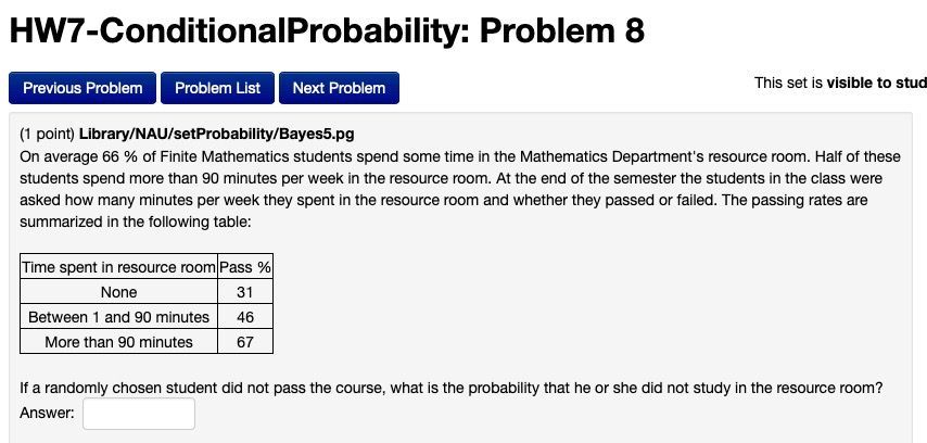
Here is a snapshot of Exercise #8 on HW7-ConditionalProbability:

HW7 #8

The first step, as usual, is to write down the given probabilities in terms of the following events:

R = “spends time in the resource room”

> 90” = “speends more than 90mins per week in the resource room”

Then the first two sentences tell us:

P(R) = 0.66  (and so P(not R) = 0.34)

P(> 90 | R) = 0.5

Then by the Multiplication Rule, we can compute P( > 90 ):

P(> 90) = P(> 90 | R) * P(R) = 0.5*0.66 = 0.33

(This should make sense from reading the first two sentences! If 66% of students spend time in the resource room, and half of those spend more than 90 minutes, then it should be clear that 33% of all students spend more than 90 minutes in the resource room.)

Now let’s look at what the exercise is asking us for: “If a randomly chosen student did not pass the course, what is the probability that he or she did not study in the resource room?”

We can rephrase this as “what is the probability that a randomly selected student did not study in the resource room given that the student did not pass the course?”, i.e., we need to calculate the conditional probability

P(not R | fail )

or, if we use “none” in place of “not R” (to match the label in the table), and use “F” for “fail“, we need to calculate:

P(not R | F)

We can do this using Bayes’ Theorem! Recall that Bayes’ Theorem gives us a way of calculating conditional probability:

Bayes Theorem

Applying this to P(not R | fail) gives us:

P(none | F) = P(F |  none)*P(none) / P(F)

We can calculate the numerator as follows:

P(F |  none) = 0.69 (since from the table, 31% of those those students who do not use the resource room pass)

and so

P(F |  none)*P(none) = 0.69*0.34

But for the denominator P(F) we need to overall percentage of students who fail, which is not immediately given in the table. We need to calculate this by accounting for the students who fail in the three different categories (events) given in the table:

  • the 69% of “none” students who fail, i.e., P(F |  none) = 0.69
  • the 54% of “1-90” students who fail, i.e., P(F |  1-90) = 0.54
  • the 33% of “>90” students who fail, i.e., P(F |  >90) = 0.33

We need to multiply each of these by the percentages of students in each category:

  • 34% of the students are in the “none” category, i.e., P(none) = 0.34
  • 33% of the students are in the “1-90” category, i.e., P(1-90) = 0.33
  • 33% of the students are in the “>90” category, i.e., P(>90) = 0.33

Then:

P(F) = P(F |  none)*P(none) + P(F |  1-90)*P(1-90) + P(F |  >90)*P(>90)

= (0.69)(0.34) + (0.54)(0.33) + (0.33)(0.33)

Thus, the solution is

P(none | F) = [0.69*0.34] / [(0.69)(0.34)+(0.54)(0.33)+(0.33)(0.33)]

Note: I will post a snapshot of a tree diagram for this exercise that may help visualize these calculations!

I will also post a note about “The Law of Total Probability” which is behind the P(F) calculation above!

Exam #2: Take-home exam due Sunday, May 3

Exam #2 is a take-home exam due Sunday; I have uploaded the pdf to Files. We also discussed some of the exam questions at the end of today’s Blackboard Collaborate class session.

As with the recent Quiz #3 and HW8, write out your solutions and submit them via Blackboard-Assignments, preferably as a single pdf file.

You will also need to submit a spreadsheet for the last exercise on the exam. As I wrote on the exam, you can either submit the spreadsheet as an additional attachment with your pdf, or you can copy/paste the share link as a comment when you submit your written solution.

Email me if you have any questions about the exam, or about related examples or exercises! I will have office hours Thursday and Friday via Blackboard Collaborate for questions (times TBA tomorrow morning).

Notes on Mon April 27 Blackboard Session / Exam #2 Announcement

On Monday we discussed the following topics:

  • 1st 30mins: we discussed the upcoming schedule of HWs and related OpenLab posts, and I announced the plan for Exam #2
    • Exam #2 will be a take-home (open book) exam which I will post later today, and will be due Sunday
    • Please join the Blackboard Collaborate session coming up today at 12p, when I will give a preview of the exam questions!
  • 30min-1h20m: we went through some examples of constructing and graphing the probability distribution of a random variables; in particular for the random variables/probability experiments of
    • X = number of heads observed when flipping a coin 3 times;
    • X = sum of two 6-sided  dice
  • 1h20m – 1h45m: we calculated the expected value E[X] of a random variable from its probability distribution

An Introduction to Bayes Theorem (including videos!)

We needed to use Bayes’ Theorem to solve HW7 #2. In this post, I try to briefly address the following questions:

  • What is Bayes’ Theorem?
  • Where does it come from?
  • What is the “Bayesian interpretation” of probability?
  • Why is called “Bayes'”  Theorem?

Also, at the bottom of the post are a handful of videos regarding Bayes Theorem (including applications to medical testing!), and links to a couple books entirely about Bayesian probability.

What is Bayes’ Theorem?

Bayes’ Theorem (or Bayes’ Rule) is following formula for computing conditional probability (screenshot taken from https://en.wikipedia.org/wiki/Bayes%27_theorem#Statement_of_theorem):

Bayes Theorem

Where does Bayes’ Theorem come from?

Where does formula above for P(A | B) come from?  We just have to do some algebra on the definition of conditional probability.

Start with the definition of conditional probability, applied to P(A | B) and P(B | A):

P(A | B) = P(A & B)/P(B)

P(B | A) = P(A & B)/P(A)

Now “clear the denominators” on the RHS of each equation by multiplying thru by P(B) and P(A), respectively:

P(A | B) * P(B) = P(A & B)

P(B | A) * P(A) = P(A & B)

Since the RHS is in both these equations, we know the two LHS of the equations are equal to each other!

P(A | B) = P(B | A) * P(A)/P(B)

Now just divide through by P(B) and we get Bayes’ Rule:

P(A | B) * P(B) = P(B | A) * P(A)


What is the “Bayesian interpretation” of probability?

Also from the wikipedia entry for Bayes’ Theorem

Bayesian Interpretation

See the wikipedia entry for Bayesian probability for more on this!


Why is it called Bayes’ Rule?

One more quote from the wikipedia entry for Bayes’ Theorem:

Bayes’ theorem is named after Reverend Thomas Bayes (/bz/; 1701?–1761), who first used conditional probability to provide an algorithm (his Proposition 9) that uses evidence to calculate limits on an unknown parameter, published as An Essay towards solving a Problem in the Doctrine of Chances (1763). In what he called a scholium, Bayes extended his algorithm to any unknown prior cause. Independently of Bayes, Pierre-Simon Laplace in 1774, and later in his 1812 Théorie analytique des probabilités, used conditional probability to formulate the relation of an updated posterior probability from a prior probability, given evidence. Sir Harold Jeffreys put Bayes’s algorithm and Laplace’s formulation on an axiomatic basis. Jeffreys wrote that Bayes’ theorem “is to the theory of probability what the Pythagorean theorem is to geometry.”


Videos on Bayes Theorem:

Here are two introductions to Bayes Theorem:


An important application of Bayes Theorem is accuracy of medical tests–this is very timely since there is a lot of discussion about the accuracy of coronavirus testing!  Here are two videos specifically on that topic:


Textbooks on Bayesian :

If you want to go even further, there are entire books devoted to Bayesian probability/statistics. Here are two introductory textbooks that look interesting (in fact, I hope to read them myself at some point!):