Homework – MATH 1372 – Ganguli

HW9, #1 and #4

Here are some hints/solutions for #1 and #4 from HW9-RandomVariables:

#1:

This exercise is really asking about permutations of the 10 students: imagine that the probability experiment consists of ordering the 10 students. The sample size is the 10! possible permutations. We go through each of the probabilities asked for:

P(X=1): What is the probability of choosing a woman first? Since there are 4 women among the 10 students, the probability of choosing a woman first is 4 out of 10, i.e., P(X=1) = 4/10.
P(X=4): For X=4, this means the first woman chosen is in the 4th position, i.e., men were chosen 1st, 2nd and 3rd, and then a woman is chosen 4th. The probability of choosing man 1st is 6/10; the subsequent (or conditional!) probability of then choosing a man 2nd is 5/9 (5 men remain among the remaining 9), and then choosing a man 3rd is 4/8 (4 men remain among the remaining 8). And then the probability of choosing one of the 4 women 4th (from the remaining 7 students) is 4/7. Thus:

P(X=4) = (6/10)*(5/9)*(4/8)*(4/7) = (6*5*4*4)/(10*9*8*7)

P(X=6): This means 5 men have been chosen for the first five positions, and then a woman is chosen 6th. Similar to above:

P(X=6) = (6/10)*(5/9)*(4/8)*(3/7)*(2/6)*(4/5) = (6*5*4*3*2*4)/(10*9*8*7*6*5)

P(X=9): For this we don’t need to do any calculations! Since there are only 6 men in class, it’s impossible that the highest ranked woman would be 9th. Even if we chose the 6 men for the first 6 positions, then we must choose a woman for 7th; i.e., 7 is the maximum possible value for X. Thus, P(X=9)=0.

#4:

One statement of this exercises reads:

“Let X represent the difference between the number of heads and the number of tails when a coin is tossed 46 times. Then P(X=12) = ?”

Note that this involves a binomial experiment with n=46 and p=0.5. But now we are interested in the random variable X = “the difference between the number of heads and the number of tails.”

When is X=12? This occurs in two separate outcomes of the binomial experiment:

when H=29 and T=17
when H=17 and T=29

We can calculate each of these binomial probabilities, either by using the binomial probability formula, or by using the spreadsheet command =binomdist(i, n, p, false). Thus, we could get P(X=12) using the spreadsheet command

=binomdist(29, 46, 0.5, false) + binomdist(17, 46, 0.5, false)

HW7 #8 (also uses Bayes’ Rule!)

Here is a snapshot of Exercise #8 on HW7-ConditionalProbability:

The first step, as usual, is to write down the given probabilities in terms of the following events:

R = “spends time in the resource room”

“> 90” = “speends more than 90mins per week in the resource room”

Then the first two sentences tell us:

P(R) = 0.66 (and so P(not R) = 0.34)

P(> 90 | R) = 0.5

Then by the Multiplication Rule, we can compute P( > 90 ):

P(> 90) = P(> 90 | R) * P(R) = 0.5*0.66 = 0.33

(This should make sense from reading the first two sentences! If 66% of students spend time in the resource room, and half of those spend more than 90 minutes, then it should be clear that 33% of all students spend more than 90 minutes in the resource room.)

Now let’s look at what the exercise is asking us for: “If a randomly chosen student did not pass the course, what is the probability that he or she did not study in the resource room?”

We can rephrase this as “what is the probability that a randomly selected student did not study in the resource room given that the student did not pass the course?”, i.e., we need to calculate the conditional probability

P(not R | fail )

or, if we use “none” in place of “not R” (to match the label in the table), and use “F” for “fail“, we need to calculate:

P(not R | F)

We can do this using Bayes’ Theorem! Recall that Bayes’ Theorem gives us a way of calculating conditional probability:

Applying this to P(not R | fail) gives us:

P(none | F) = P(F | none)*P(none) / P(F)

We can calculate the numerator as follows:

P(F | none) = 0.69 (since from the table, 31% of those those students who do not use the resource room pass)

and so

P(F | none)*P(none) = 0.69*0.34

But for the denominator P(F) we need to overall percentage of students who fail, which is not immediately given in the table. We need to calculate this by accounting for the students who fail in the three different categories (events) given in the table:

the 69% of “none” students who fail, i.e., P(F | none) = 0.69
the 54% of “1-90” students who fail, i.e., P(F | 1-90) = 0.54
the 33% of “>90” students who fail, i.e., P(F | >90) = 0.33

We need to multiply each of these by the percentages of students in each category:

34% of the students are in the “none” category, i.e., P(none) = 0.34
33% of the students are in the “1-90” category, i.e., P(1-90) = 0.33
33% of the students are in the “>90” category, i.e., P(>90) = 0.33

Then:

P(F) = P(F | none)*P(none) + P(F | 1-90)*P(1-90) + P(F | >90)*P(>90)

= (0.69)(0.34) + (0.54)(0.33) + (0.33)(0.33)

Thus, the solution is

P(none | F) = [0.69*0.34] / [(0.69)(0.34)+(0.54)(0.33)+(0.33)(0.33)]

Note: I will post a snapshot of a tree diagram for this exercise that may help visualize these calculations!

I will also post a note about “The Law of Total Probability” which is behind the P(F) calculation above!

HW7 #2 (using Bayes’ Rule)

Here is a snapshot of Exercise #2 on HW7-ConditionalProbability:

The first step with this exercise is to write down the given probabilities in terms of events that we can call:

W = neighbor waters the plant

D = plant dies

So we are given the following in the statement of the problem:

P( D | W ) = 0.5 (and so P( not D | W ) = 1 – 0.5 = 0.5)

P( D | not W ) = 0.85 (and so P( not D | W ) = 1 – 0.85 = 0.15)

Also we are given P(W) = 0.83 (and so P(not W) = 1 – 0.83 = 0.17)

We can arrange these into a tree diagram, and also use the Multiplication Rule along the branches of the tree to compute the “joint probabilities”:

P(W & D) = P(W) * P(D | W) = (0.83)(0.5) = 0.415

P(W & not D) = P(W) * P(not D | W) = (0.83)(0.5) = 0.415

P(not W & D) = P(not W) * P(D | not W) = (0.17)(0.85) = 0.1445

P(not W & not D) = P(not W) * P(not D | not W) = (0.17)(0.15) = 0.0255

(Note that these four add up to 1, as they should, since these 4 combinations cover the 4 possible outcomes! You can think of this as a probability distribution over these 4 possible outcomes.)

A tricky part of this question is interpreting what probability the question is asking for. It turns out that “What is the probability that the plant died because neighbor forgot to water it?” corresponds to P(not W | D)!

In order to compute this probability from the given probabilities, we need to apply what’s called Bayes’ Theorem, which comes from the definition of conditional probability.

(See this post for a longer introduction to Bayes’ Theorem, including its algebraic derivation from the definition of conditional probability.)

Here is a statement of Bayes’ Theorem, taken from https://en.wikipedia.org/wiki/Bayes%27_theorem#Statement_of_theorem:

We can apply Bayes’ Theorem this to compute P(not W | D); here is the tree diagram and the calculation of P(not W | D) (in the bottom left part of the page):

Exercise: Probability Distribution (X = sum of two 6-sided dice)

We have previously discussed the probability experiment of rolling two 6-sided dice and its sample space. Now we can look at random variables based on this probability experiment. A natural random variable to consider is:

X = sum of the two dice

You will construct the probability distribution of this random variable. For reference, I wrote out the sample space and set up the probability distribution of X; see the snapshot below.

It will be a exam exercise to complete the probability distribution (i.e., fill in the entries in the table below) and to graph the probability distribution (i.e., as a histogram):

Sample space of rolling two 6-sided dice

Notes for Mon April 20 / HW8 (Permutations & Combinations)

Here’s a brief recap of today’s Blackboard Collaborate session:

For the first approximately 40mins, we gave an overview of HW8, which consists of permutations and combinations calculations:

HW8 is a written homework assignment; you can find the pdf with the homework exercises under Files
- HW8 is due next Monday (April 27)
- I will create an Assignment in Blackboard where you can submit your solutions (preferably as a pdf, as you did for Quiz #3 over the weekend)
- we went through HW8 #1 together–in particular I wanted to demonstrate how to show your work;
- we will go through at least one more exercise from HW8 during Wednesday’s Blackboard session

We spent the remaining hour reviewing random variables and introducing probability distributions for such random variables.

Please review the Class Outline on those topics–in particular, it’s essential you understand the example involving the probability experiment of flipping a coin 3 times, and constructing the probability distribution for the random variable “X = the number of heads observed.” We will build on that example when we discuss binomial experiments and binomial random variables.

You can review the Blackboard recording, and/or you can view this Khan Academy video, which constructs the probability distribution for that same random variable:

WebWork Hints: Conditional Probability (HW6 & HW7)

Here are recaps of the WebWork exercises we went over in the Blackboard Collaborate class session earlier today (remember that you can view the recording of the BB Collaborate session at https://us-lti.bbcollab.com/recording/dda6c10a1bf645ac99623a8f9549af40).

(If you catch any errors in my solutions below, please let me know!)

HW6:

#16: We went over #16 first–it helps to understand these tree diagrams before doing #15 (below).

Here’s the tree diagram from#16 (the probabilities on your tree may be different):

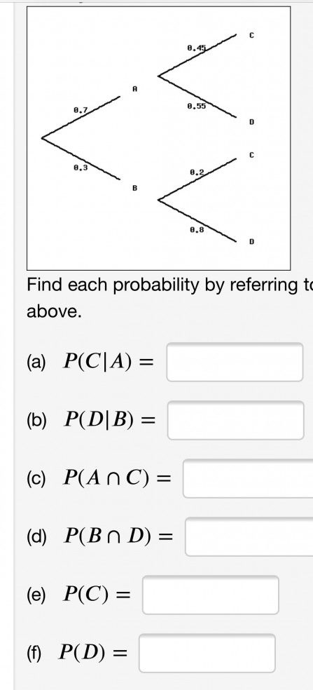
As we discussed, the tree diagram shows various probabilities for a certain probability experiment, which you can think of as two sequential coin flips:

the first coin flip comes up as A or B, with probabilities 0.7 and 0.3, respectively (think of this as a weighted coin!)
the second coin flip comes up as C or D–but the probabilities depend on whether the first coin flip came up A or B!
- in particular, the conditional probability P(C|A) means the probability of C given that A has occurred, i.e., P(C|A) is the number attached to the branch that leads to C from A. Thus, in this example, P(C|A) = 0.45.
- Similarly, you can read off P(D|A), P(C|B) and P(D|B) directly from the tree diagram: 0.55, 0.2, and 0.8 respectively.
- You can compute probabilities such P(A∩C) and P(B∩D) by using the Multiplication Rule. If we write it out for P(A∩C):
  - P $P (A \cap C) =$
- Finally, to compute P(C), add up the probabilities of the two different paths that lead to the outcome C, i.e., via A or via B:
  - P(C) = P $P (A \cap C) =$ P $P (A \cap C) =$ $P (A \cap C) =$

#15:

Note the hint at the bottom: draw a tree diagram, like the one we saw in #16!

The probability experiment here involves choosing a randomly selected person over 40. But if you look at the questions you’re asked in (a), (b), (c), we can interpret the two “coin flips” upon selecting a person as

(1) does that person have diabetes or not; and

(2) is that person diagnosed as having diabetes or not (we can call these two outcomes as “testing positive” or “testing negative”)

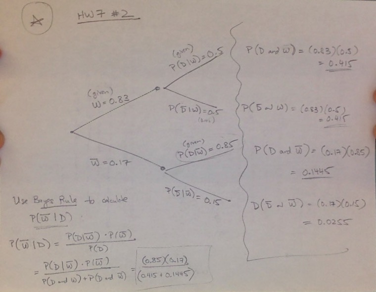
Here’s a snapshot of the tree diagram I drew, with probabilities pulled from the percentages given in the statement of the exercise:

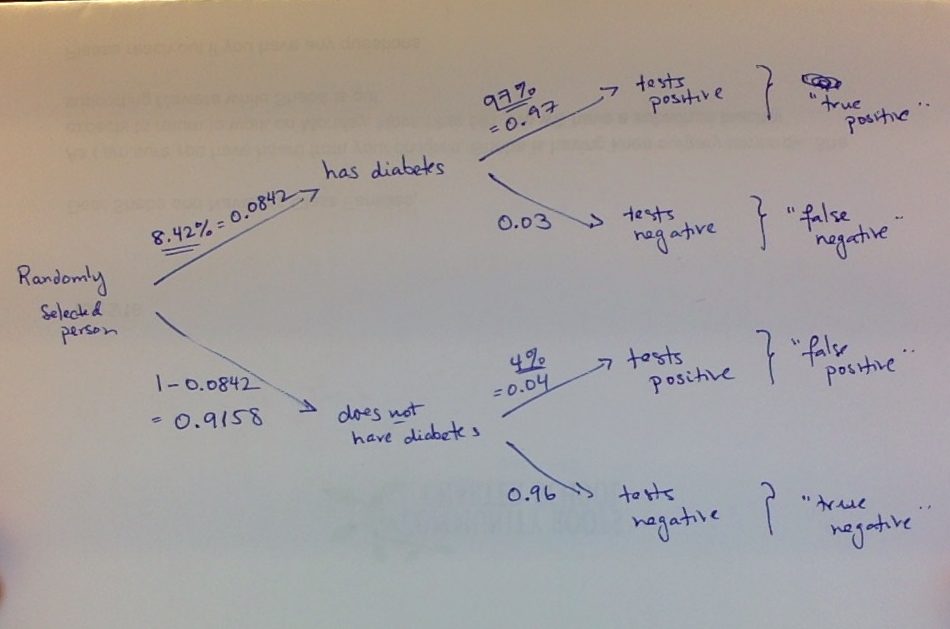
Note that I got the underlined percentages/probabilities directly from the statement of the exercise, and calculated the other ones by subtraction from 1 (e.g., we are told that 8.42% of Americans have diabetes, so 100% – 8.42% = 91.58% do not have diabetes. These are the two probabilities shown on the “first branch”–whether the randomly selected person has diabetes or not.)

Now we can just calculate the answers from this tree (as we did for #16):

a) the probability of a false positive, i.e., P( “does not have diabetes” & “tests positive”) is the product of the probabilities along that branch:

P( “does not have diabetes” & “tests positive”)= (0.9158)(0.04)

b) To find the probability that a randomly selected adult of $40$ is diagnosed as not having diabetes, i.e., P(“tests negative”), we need to add together the probabilities of travelling along the two paths that lead to that outcome (i.e., (1) has diabetes & tests negative + (2) does not have diabetes & tests negative):

P(“tests negative”) = P(“has diabetes” & “tests negative”) + P(“does not have diabetes” & “tests negative”) = (0.9158)(0.96) + (0.0842)(0.03)

[you should see how these numbers come from following the paths!]

(c) is trickier: note that the words “given that” mean we have to calculate the following conditional probability: P(“has diabetes” | “tests negative”)

By the definition of conditional probability:

P(“has diabetes” | “tests negative”) =

P(“has diabetes” & “tests negative”) / P(“tests negative”)

We get the numerator from multiplying the probabilities along that path:

P(“has diabetes” & “tests negative”) = (0.0842)(0.03)

and we already calculated the denominator in (b)!

P(“has diabetes” | “tests negative”) =

P(“has diabetes” & “tests negative”) / P(“tests negative”) =

(0.0842)(0.03)/[(0.9158)(0.96) + (0.0842)(0.03)]

HW7:

#1: This is similar to #16 from HW6! See the solutions above.

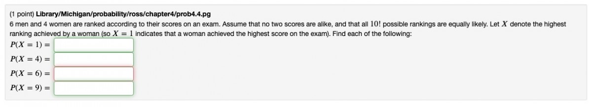
#3: The statement of the exercise reads: “Two cards are drawn from a regular deck of 52 cards, without replacement. What is the probability that the first card is an ace of clubs and the second is black?”

This is an application of conditional probability and the Multiplication Rule. First, recall that “without replacement” means that after drawing the 1st card, you don’t put it back it in the deck–so you’re sample space for the 2nd draw is reduced to 51 cards.

We need to calculate the probability

P( “1st card is ace of clubs” & “2nd card black”) =

P(“1st card ace of clubs”) * P(“2nd card black”| “1st card is ace of clubs”) =

(1/52)*(25/51)

Note that the P(“2nd card black”| “1st card is ace of clubs”) = 25/51 because the sample space is reduced to the remaining 51 cards, and of those only 25 are black (b/c we are assuming the 1st card drawn was the ace of clubs, which is black).

Also note that we can do a rough estimation of this probability, as follows:

1/52 ≈ 0.02 (actually slightly less than 0.02, since 1/50 = 0.02) and

25/51 ≈ 1/2 (actually slightly less than 1/2, since 25/50 = 1/2)

so (1/52)*(25/51) ≈ 0.02*(1/2) = 0.01

So we can estimate that the probability of drawing an ace of clubs and then a black card is less than 0.01, i.e., less than 1%.

(Using a calculator, the exact value is

(1/52)*(25/51) = 25/(52*51) = 0.00942684766214178, i.e., 0.942.. %)

#6: My statement of the exercise reads “Of 380 male and 220 female employees at the Flagstaff Mall, 250 of the men and 130 of the women are on flex-time (flexible working hours). Given that an employee selected at random from this group is on flex-time, what is the probability that the employee is a woman? ”

This is a straightforward conditional probability calcuation; you are being asked to calculate P(“woman”|”flex-time”); the “reduced sample space” for calculating this conditional probability is the number of flex-time employees, which in this example is 250+130 = 380. The number of women in this reduced sample space is 130 (the number of women on flex-time).

Hence,

P(“woman”|”flex-time”) = 130/280 = 13/28.

If you want to apply the formula for conditional probability, you can get to the solution that way. Actually it is instructive to see how that works:

P(“woman”|”flex-time”) = P(“woman” & “flex-time”)/P(“flex-time”) = (130/600)/(280/600) = (130/600)*(600/280) = 130/280.

Note that the probabilities here are relative to the original sample space of 380+220 = 600 total employees, which is why that is in the denominators for P(“woman” & “flex-time”) and P(“flex-time”); but when we do the division, those terms cancel out!

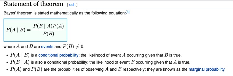
#7: You are given the values of P(E∩F), P(E|F) and P(F|E). To calculate P(E) and P(F) from these values, recall the formula for the conditional probabilities:

(1) P(E|F) = P(E∩F)/P(F)

(2) P(F|E) = P(E∩F)/P(E)

If you solve these equations for P(F) and P(E) respectively, you get:

(1a) P(F) = P(E∩F)/P(E|F)

(2a) P(E) = P(E∩F)/P(E|F)

[You should understand the algebra for getting from (1) to (1a), and from (2) to (2a)! It’s pretty simple algebra–it’s just solving x = y/z for z, i.e., z = y/x.]

Now you can use (1a) and (2a) to calculate P(F) and P(E).

Then you can solve for P(E∪F) using the Addition Rule:

P(E∪F) = P(E) + P(F) – P(E∩F)

WebWork: HW6 Hints

I received a couple questions about HW6 exercises earlier this week; I thought it might be helpful to post my solutions below. Even if you have already completed these exercises, it might be worth your time to read my solutions, to see how I set up the problem and how I write out the solution.

I will update this post with some hints to the last couple exercises on HW6, since I see that many of you have completed all but the last couple exercises.

I will also start writing up some hints to the HW7 exercises shortly. Check back here for an update.

PS: Please feel free to e-mail me homework questions like this!

Someone in the class e-mailed me the following screenshot of their HW6, Problem 2:

WebWork HW6, Exercise 2

Here is my solution:

WebWork HW6, Exercise 2 Solution

Here is a screenshot of HW6, Problem 8:

WebWork HW6, Exercise 8

with my solution:

WebWork: HW6 Exercise 8 - Solution

Here is a screenshot of HW6, Problem 6:

HW6, Problem 6

First let’s think about the sample space for a family with 5 children–what are the different gender possibilities? (Taking into account birth order!)

This is basically the same as a previous type of probability experiment we’ve discussed–flipping a coin 5 times! We have 2^5 = 32 possible outcomes in the sample space:

S = { GGGGG, GGGGB, GGGBG, …. , BBBBB}

Each of these is equally likely, but additionally we are told that we know the family has at least one girl. Hence we can rule out “BBBBB” (5 boys), and so the “reduced” sample space has 31 possibilities.

Hence, the probability of 5 girls is 1/31 (since there is obviously only one outcome with 5 girls: “GGGGG”).

Note that we can frame this as a conditional probability! We have calculated

P( GGGGG | at least one girl )

Category: Homework