Video: “Exponential growth and epidemics”

Here is a 9min video that I highly recommend you watch:

You can get a lot out of just watching the first minute: watch how he steps up the graph of the # of COVID-19 cases (outside mainland China) from Jan 22 to March 6, and shows that C(n+1) ≈ 1.2*C(n), i.e., we’re seeing exponential growth with C(n) = C(0)*(1.2)^n. Note that he has the advantage that he can just “zoom out” to redraw the scale of the y-axis.

After that initial segment, he starts discussing some parameters relevant to the topics of our course (“E = Average number of people someone infected is exposed to each day,” and “p = Probability of each exposure becoming an infection”).

Also starting at around 1:50 mark, he shows what a logarithmic scale is, and why it’s useful for graphing exponential growth curves–they turn into straight lines on a log scale! And then he does a linear regression, and shows the R^2 (the coefficient of determination!)

“What Worked in 1918-1919?”

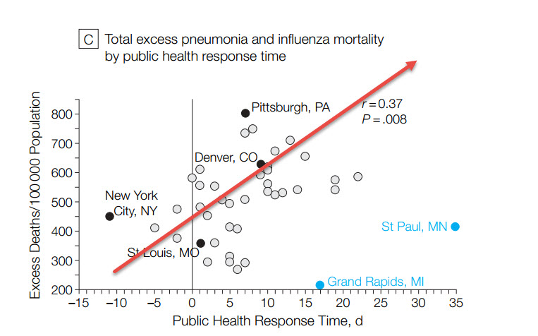
Here is a scatterplot from a March 7 blog post titled “What Worked in 1918-1919?“:

1918 flu: excess mortality vs public health response time

Here is the intro to this graph from the Marginal Revolution blog post:

Marginal Revolution blog post

Take a look at the 2007 paper (“Nonpharmaceutical Interventions Implemented by US Cities During the 1918-1919 Influenza Pandemic“) which contains a number of additional scatterplots!

Interpreting the linear regression parameters

Yesterday in class I discussed how we can interpret the linear regression parameters (i.e., the y-intercept a (“alpha”) and the slope (“beta”) yielding a linear regression line (or what we also call a “linear model”)

y = a + bx

See below for a summary (you can also take a look at the Khan Academy videos “Interpreting y-intercept in regression” and “Interpreting slope in regression“):

  • Recall that the linear model is used to predict an “output” value y for a given “input” value x
  • In terms of the line, the y-intercept a is the y-value where the line intersects the x-axis, i.e., when x = 0.  Thus, in terms of the linear regression model, the y-intercept a is the predicted value of the dependent variable y when the independent variable x is 0.
  • In terms of the line, the slope b is how much y increases or decreases if x is increased by 1.  Thus, in terms of the linear regression model, the slope b is the predicted change in the dependent variable y if the independent variable x is increased by 1.

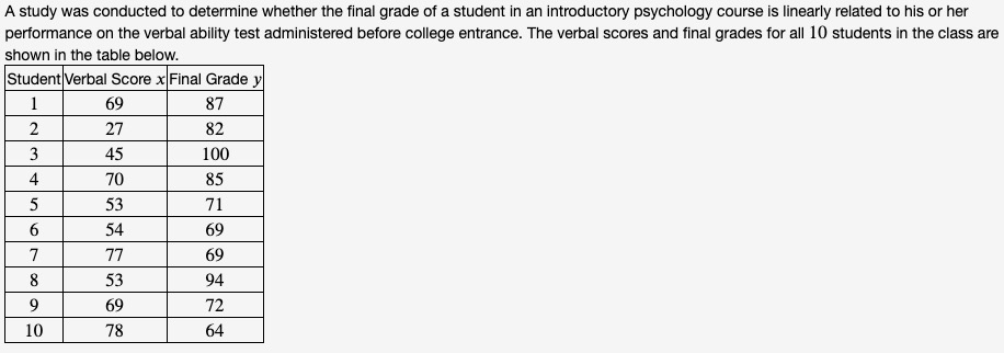
For example, this was an exercise on the “HW4-Paired Data” WebWork set:

Paired data set from WebWork HW4
Exercise from WebWork “HW4-Paired Data”

The results of linear regression for this data set (i.e., regressing the dependent variable y (final grade) on the independent variable x (verbal score) yield the linear regression parameters:

  • y-intercept a ≈ 99.1 ; this can be interpreted as the predicted final grade of a student who gets a verbal score of 0
  • slope b ≈ -0.333 ; this can be interpreted as saying that a student who increases their verbal score by 1 will decrease their final grade by -0.333