HW7 #2 (using Bayes’ Rule)

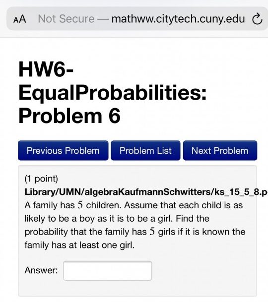
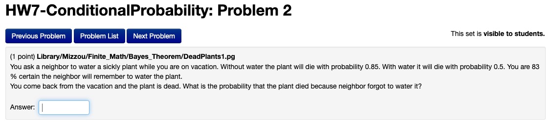
Here is a snapshot of Exercise #2 on HW7-ConditionalProbability:

HW7-2

The first step with this exercise is to write down the given probabilities in terms of events that we can call:

W = neighbor waters the plant

D = plant dies

So we are given the following in the statement of the problem:

P( D | W ) = 0.5 (and so P( not D | W  ) = 1 – 0.5 = 0.5)

P( D | not W ) = 0.85 (and so P( not D | W ) = 1 – 0.85 = 0.15)

Also we are given P(W) = 0.83 (and so P(not W) = 1 – 0.83 = 0.17)

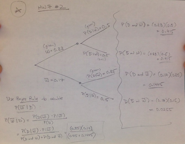
We can arrange these into a tree diagram, and also use the Multiplication Rule along the branches of the tree to compute the “joint probabilities”:

P(W & D) =  P(W) * P(D | W) = (0.83)(0.5) = 0.415

P(W & not D) = P(W) * P(not D | W) = (0.83)(0.5) = 0.415

P(not W & D) = P(not W) * P(D | not W) = (0.17)(0.85) = 0.1445

P(not W & not D) = P(not W) * P(not D | not W) = (0.17)(0.15) = 0.0255

(Note that these four add up to 1, as they should, since these 4 combinations cover the 4 possible outcomes! You can think of this as a probability distribution over these 4 possible outcomes.)

A tricky part of this question is interpreting what probability the question is asking for. It turns out that “What is the probability that the plant died because neighbor forgot to water it?” corresponds to P(not W | D)!

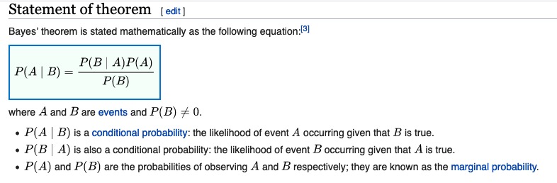
In order to compute this probability from the given probabilities, we need to apply what’s called Bayes’ Theorem, which comes from the definition of conditional probability.

(See this post for a longer introduction to Bayes’ Theorem, including its algebraic derivation from the definition of conditional probability.)

Here is a statement of Bayes’ Theorem, taken from https://en.wikipedia.org/wiki/Bayes%27_theorem#Statement_of_theorem:

Bayes Theorem

We can apply Bayes’ Theorem this to compute P(not W | D); here is the tree diagram and the calculation of P(not W | D) (in the bottom left part of the page):

HW7 #2: Solution

Exercise: Probability Distribution (X = sum of two 6-sided dice)

We have previously discussed the probability experiment of rolling two 6-sided dice and its sample space.  Now we can look at random variables based on this probability experiment. A natural random variable to consider is:

X = sum of the two dice

You will construct the probability distribution of this random variable. For reference, I wrote out the sample space and set up the probability distribution of X; see the snapshot below.

It will be a exam exercise to complete the probability distribution (i.e., fill in the entries in the table below) and to graph the probability distribution (i.e., as a histogram):

Sample space of rolling two 6-sided dice

WebWork: HW6 Hints

I received a couple questions about HW6 exercises earlier this week; I thought it might be helpful to post my solutions below.  Even if you have already completed these exercises, it might be worth your time to read my solutions, to see how I set up the problem and how I write out the solution.

I will update this post with some hints to the last couple exercises on HW6, since I see that many of you have completed all but the last couple exercises.

I will also start writing up some hints to the HW7 exercises shortly. Check back here for an update.

PS: Please feel free to e-mail me homework questions like this!


Someone in the class e-mailed me the following screenshot of their HW6, Problem 2:

WebWork HW6, Exercise 2

Here is my solution:

WebWork HW6, Exercise 2 Solution


Here is a screenshot of HW6, Problem 8:

WebWork HW6, Exercise 8

with my solution:

WebWork: HW6 Exercise 8 - Solution


Here is a screenshot of HW6, Problem 6:

HW6, Problem 6

First let’s think about the sample space for a family with 5 children–what are the different gender possibilities? (Taking into account birth order!)

This is basically the same as a previous type of probability experiment we’ve discussed–flipping a coin 5 times! We have 2^5 = 32 possible outcomes in the sample space:

S = { GGGGG, GGGGB, GGGBG, …. , BBBBB}

Each of these is equally likely, but additionally we are told that we know the family has at least one girl. Hence we can rule out “BBBBB” (5 boys), and so the “reduced” sample space has 31 possibilities.

Hence,  the probability of 5 girls is 1/31 (since there is obviously only one outcome with 5 girls: “GGGGG”).

Note that we can frame this as a conditional probability! We have calculated

P( GGGGG | at least one girl )

Conditional Probability

This past Monday, we introduced conditional probability in our Blackboard Collaborate session.  Here is a brief recap, with some online resources included below that go over the definition and go through some examples.

The conditional probability of A given B is defined as:

P(A|B) = P(A & B)/P(B)

Note that by switching A and B, we can also look at the conditional probability of B given A:

P(B|A) = P(A & B)/P(A)

(Note that the numerator is the same in both cases, since P(A&B) = P(B&A).  The denominator is the probability of the “condition” i.e., the event after the vertical line “|”.)

The following 2 videos may be helpful:

If you have a copy of the textbook (Ross), you should read the examples listed on the class outline pdf.  I will try to update this post with some additional online examples shortly.