HW7 #8 (also uses Bayes’ Rule!)

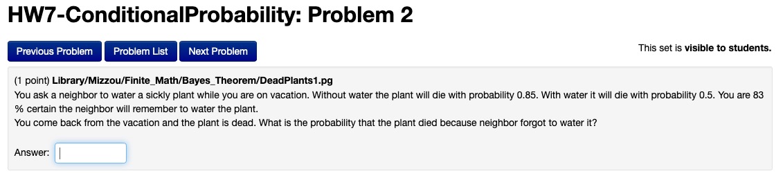
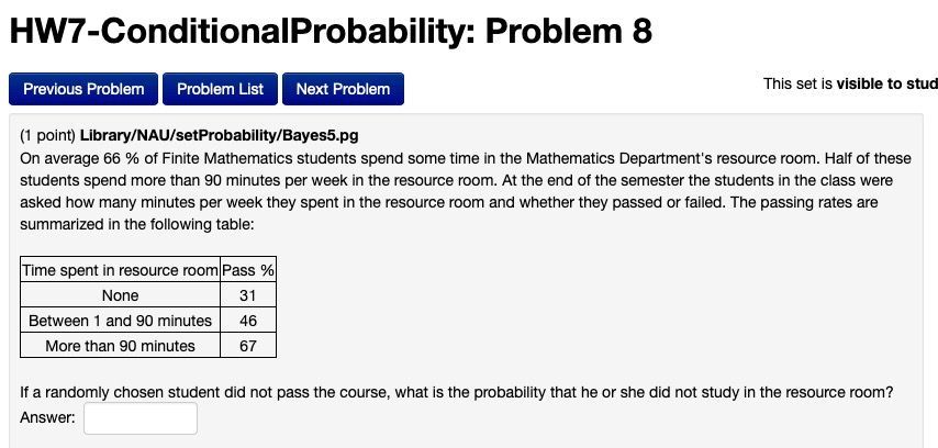
Here is a snapshot of Exercise #8 on HW7-ConditionalProbability:

HW7 #8

The first step, as usual, is to write down the given probabilities in terms of the following events:

R = “spends time in the resource room”

> 90” = “speends more than 90mins per week in the resource room”

Then the first two sentences tell us:

P(R) = 0.66  (and so P(not R) = 0.34)

P(> 90 | R) = 0.5

Then by the Multiplication Rule, we can compute P( > 90 ):

P(> 90) = P(> 90 | R) * P(R) = 0.5*0.66 = 0.33

(This should make sense from reading the first two sentences! If 66% of students spend time in the resource room, and half of those spend more than 90 minutes, then it should be clear that 33% of all students spend more than 90 minutes in the resource room.)

Now let’s look at what the exercise is asking us for: “If a randomly chosen student did not pass the course, what is the probability that he or she did not study in the resource room?”

We can rephrase this as “what is the probability that a randomly selected student did not study in the resource room given that the student did not pass the course?”, i.e., we need to calculate the conditional probability

P(not R | fail )

or, if we use “none” in place of “not R” (to match the label in the table), and use “F” for “fail“, we need to calculate:

P(not R | F)

We can do this using Bayes’ Theorem! Recall that Bayes’ Theorem gives us a way of calculating conditional probability:

Bayes Theorem

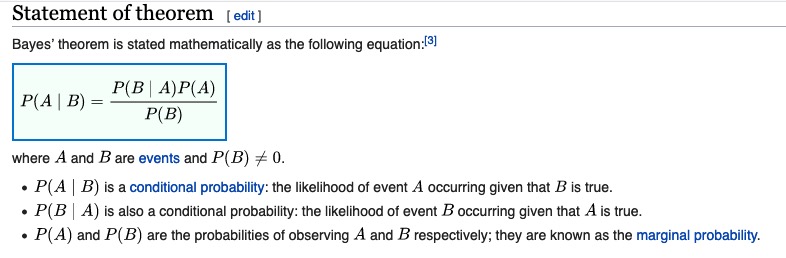
Applying this to P(not R | fail) gives us:

P(none | F) = P(F |  none)*P(none) / P(F)

We can calculate the numerator as follows:

P(F |  none) = 0.69 (since from the table, 31% of those those students who do not use the resource room pass)

and so

P(F |  none)*P(none) = 0.69*0.34

But for the denominator P(F) we need to overall percentage of students who fail, which is not immediately given in the table. We need to calculate this by accounting for the students who fail in the three different categories (events) given in the table:

  • the 69% of “none” students who fail, i.e., P(F |  none) = 0.69
  • the 54% of “1-90” students who fail, i.e., P(F |  1-90) = 0.54
  • the 33% of “>90” students who fail, i.e., P(F |  >90) = 0.33

We need to multiply each of these by the percentages of students in each category:

  • 34% of the students are in the “none” category, i.e., P(none) = 0.34
  • 33% of the students are in the “1-90” category, i.e., P(1-90) = 0.33
  • 33% of the students are in the “>90” category, i.e., P(>90) = 0.33

Then:

P(F) = P(F |  none)*P(none) + P(F |  1-90)*P(1-90) + P(F |  >90)*P(>90)

= (0.69)(0.34) + (0.54)(0.33) + (0.33)(0.33)

Thus, the solution is

P(none | F) = [0.69*0.34] / [(0.69)(0.34)+(0.54)(0.33)+(0.33)(0.33)]

Note: I will post a snapshot of a tree diagram for this exercise that may help visualize these calculations!

I will also post a note about “The Law of Total Probability” which is behind the P(F) calculation above!

HW7 #2 (using Bayes’ Rule)

Here is a snapshot of Exercise #2 on HW7-ConditionalProbability:

HW7-2

The first step with this exercise is to write down the given probabilities in terms of events that we can call:

W = neighbor waters the plant

D = plant dies

So we are given the following in the statement of the problem:

P( D | W ) = 0.5 (and so P( not D | W  ) = 1 – 0.5 = 0.5)

P( D | not W ) = 0.85 (and so P( not D | W ) = 1 – 0.85 = 0.15)

Also we are given P(W) = 0.83 (and so P(not W) = 1 – 0.83 = 0.17)

We can arrange these into a tree diagram, and also use the Multiplication Rule along the branches of the tree to compute the “joint probabilities”:

P(W & D) =  P(W) * P(D | W) = (0.83)(0.5) = 0.415

P(W & not D) = P(W) * P(not D | W) = (0.83)(0.5) = 0.415

P(not W & D) = P(not W) * P(D | not W) = (0.17)(0.85) = 0.1445

P(not W & not D) = P(not W) * P(not D | not W) = (0.17)(0.15) = 0.0255

(Note that these four add up to 1, as they should, since these 4 combinations cover the 4 possible outcomes! You can think of this as a probability distribution over these 4 possible outcomes.)

A tricky part of this question is interpreting what probability the question is asking for. It turns out that “What is the probability that the plant died because neighbor forgot to water it?” corresponds to P(not W | D)!

In order to compute this probability from the given probabilities, we need to apply what’s called Bayes’ Theorem, which comes from the definition of conditional probability.

(See this post for a longer introduction to Bayes’ Theorem, including its algebraic derivation from the definition of conditional probability.)

Here is a statement of Bayes’ Theorem, taken from https://en.wikipedia.org/wiki/Bayes%27_theorem#Statement_of_theorem:

Bayes Theorem

We can apply Bayes’ Theorem this to compute P(not W | D); here is the tree diagram and the calculation of P(not W | D) (in the bottom left part of the page):

HW7 #2: Solution

Exercise: Probability Distribution (X = sum of two 6-sided dice)

We have previously discussed the probability experiment of rolling two 6-sided dice and its sample space.  Now we can look at random variables based on this probability experiment. A natural random variable to consider is:

X = sum of the two dice

You will construct the probability distribution of this random variable. For reference, I wrote out the sample space and set up the probability distribution of X; see the snapshot below.

It will be a exam exercise to complete the probability distribution (i.e., fill in the entries in the table below) and to graph the probability distribution (i.e., as a histogram):

Sample space of rolling two 6-sided dice

Notes for Mon April 20 / HW8 (Permutations & Combinations)

Here’s a brief recap of today’s Blackboard Collaborate session:

For the first approximately 40mins, we gave an overview of HW8, which consists of permutations and combinations calculations:

  • HW8 is a written homework assignment; you can find the pdf with the homework exercises under Files
    • HW8 is due next Monday (April 27)
    • I will create an Assignment in Blackboard where you can submit your solutions (preferably as a pdf, as you did for Quiz #3 over the weekend)
    • we went through HW8 #1 together–in particular I wanted to demonstrate how to show your work;
    • we will go through at least one more exercise from HW8 during Wednesday’s Blackboard session

We spent the remaining hour reviewing random variables and introducing probability distributions for such random variables.

Please review the Class Outline on those topics–in particular, it’s essential you understand the example involving the probability experiment of flipping a coin 3 times, and constructing the probability distribution for the random variable “X = the number of heads observed.”  We will build on that example when we discuss binomial experiments and binomial random variables.

You can review the Blackboard recording, and/or you can view this Khan Academy  video, which constructs the probability distribution for that same random variable: