Morphometrics and physical markers

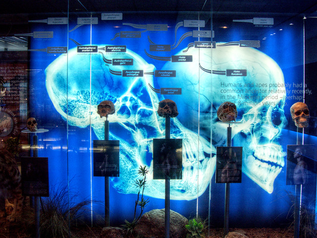
Morphometrics (morpho– shape; metrics– measurements) is the use of physical measurements to determine the relatedness of organisms. With extinct organisms that have died out long ago, DNA extraction proves to be difficult. Likewise, prior to DNA technologies to analyze species, Linnean taxonomy was ascribed to organisms based on similarities in features.

Describing Species and Variation of Morphologies

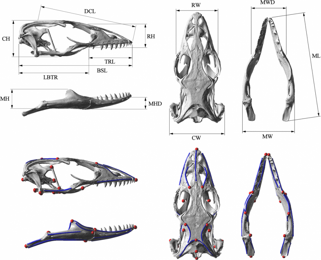
Below are images of skull landmarks of the lizard family Varanidae. This family includes monitor lizards and Komodo Dragons.As can be seen below, the general morphology of the skulls are similar enough that they all retain the same landmarks. The figure below also illustrates the diversity in these lizards that illustrate a large variety between species.

Landmarks Standardize measurements

Having a set of shared landmarks provides the opportunity to make systematic measurements of morphometric features.

 

Euclidean distance to measure relatedness

Euclidean distance is a measurement derived from Pythagorean geometry that describes the shortest distance (d) between 2 points (A & B) as a straight line using triangulation. In a cartesian space, the points can be defined:

and 

Standard pythagorean theorem can be expressed as:

To find the distance between the 2 points, we utilize algebra to calculate for .

In this case, we expand to comparing the coordinates of the two points:

and

We can then expand this idea to include the differences of data points that describe the comparisons of multiple measurements.

Calculating distance with R

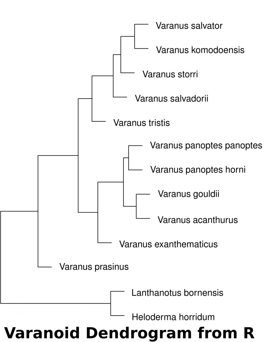
1. Download the dataset (McCurry et al. 2015) associated with this activity (a Comma Separated Value .csv file). This can be used in a spreadsheet or in a text editor. This data can be imported into R to determine the euclidean distances of landmarks.
2. The following code in R will download the data set into a variable called “varanoid”, measure euclidean distance and save a plot into a PDF file in a directory called “/tmp”.

## install curl for fetching from internet if it isn't
install.packages('curl')
## Load the curl library
library(curl)
## read the data of measurements and assign it to a variable 'varanoid'
varanoid = read.csv(curl('https://raw.githubusercontent.com/jeremyseto/bio-oer/master/data/varanoid.csv'))
## set the row names to the Species column
row.names(varanoid) = varanoid$Species
## remove the first column of the table to have purely numeric data
varanoid_truncated = (varanoid[,2:14])
## calculate distance using euclidean as the method
dist_measure = dist(varanoid_truncated, method='euclidean')
## display dist_measure to look at the comparisons
dist_measure
varanoid_cluster = hclust(dist_measure)
## open PDF as a graphics device  to save a file in the '/tmp' directory
pdf(file='/tmp/varanoid_tree.pdf')
plot(varanoid_cluster)
dev.off()
## close the device to save the plot as pdf

 

 

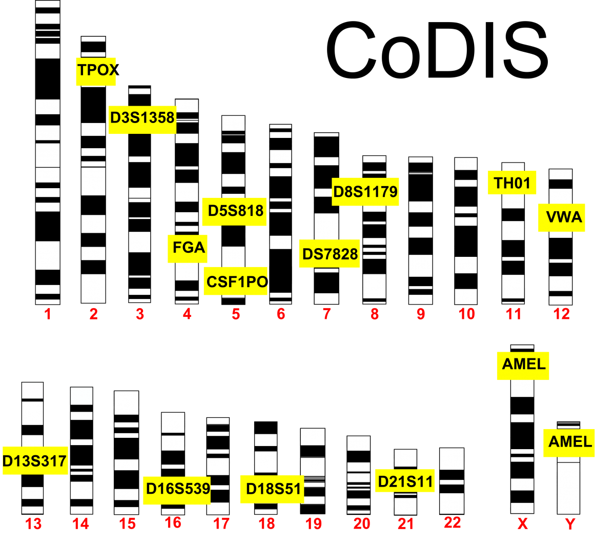
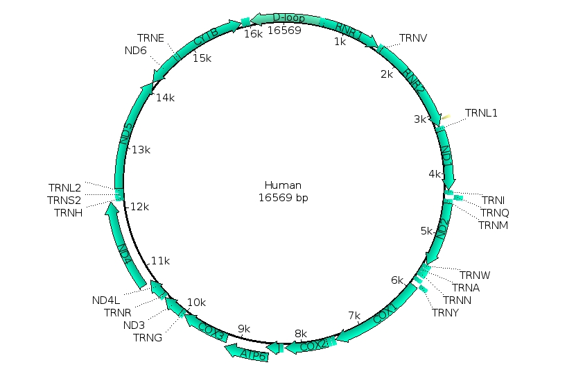
DNA Analysis

Before starting this activity, review bioinformatics and sequence analysis.

1. Search NCBI for mitochondrial sequences from the species involved in McCurry 2015. The data has been submitted by Ast (2001).
2. Find the sequences and identify/extract elements that are common to all
3. Assemble the shared sequences in a text editor as a single FASTA file where each species is separated by a header (“>Species A”)
   • Notepad on Windows (but it’s better to download notepad++)
   • Textedit on Mac (but probably better to download TextWrangler)
   • Gedit on Linux
4. Save the file as “something.fasta”
5. Perform a multiple sequence analysis using UGENE
6. Generate a phylogenetic tree using UGENE. For this exercise, use Maximum Likelihood (PhyML) as the algorithm. File the tutorial below.
7. Compare the DNA with the morphometric analyses. What problems could we imagine arise if we rely solely on morphometry.

References

• McCurry MR, Mahony M, Clausen PD, Quayle MR, Walmsley CW, Jessop TS, Wroe S, Richards H, McHenry CR. (2015) The Relationship between Cranial Structure, Biomechanical Performance and Ecological Diversity in Varanoid Lizards. PLoS ONE 10(6): e0130625. doi: 10.1371/journal.pone.0130625
• Ast, Jennifer C. (2001) Mitochondrial DNA Evidence and Evolution in Varanoidea (Squamata). Cladistics 17(3): 211–26.  http://www.sciencedirect.com/science/article/pii/S0748300701901690
• Fisher, R.A. (1936) The use of multiple measurements in taxonomic problems.  Annals of Eugenics, 7: 179–188. doi:10.1111/j.1469-1809.1936.tb02137.x

Tags: analysis, visual communication, integration of knowledge, breadth of knowledge, quantitative reasoning

Genetic Manipulation (selection)

Genetic modification of organisms has been occurring through human manipulation since the beginning of agriculture. Humans selectively bred crops and livestock to propagate desirable traits in a process termed artificial selection. The original grass that gave rise to domesticated corn called teosinte hardly resembles what we think of when imagining modern maize.

Variation: Crop domestication

Selective breeding can yield a variety of features even within the same species. Below is selection of vegetables of the species Brassica oleracea that have been developed into different varieties over the course of agricultural history.

Variation: Animal domestication

Companion animals like dogs underwent thousands of years of domestication and selection for traits that were desirable for different circumstances. A high degree of morphological diversity exists between dog breeds and their ancestral grey wolf progenitor.

Genetic Manipulation (engineered)

Artificial selection takes multiple generations over a long period of time. With the advent of recombinant DNA and biotechnology, scientists can now genetically modify organisms through introduction of foreign genes to provide desirable characteristics within one generation. This process does not require traits to naturally arise in a species.

GloFish® are novelty pets that have the insertion of various cnidarian fluorescent protein genes into the genome. These fish were released in the United States in 2003 and have subsequently been developed in red, orange, and blue varieties. Black tetras and tiger barbs are also now available.

Tags: integration of knowledge, life-long learning, breadth of knowledge

The PCR amplification of the mitochondrial control region

There are 2 hypervariable regions within the control region of the mitochondria. This exercise amplifies just one of these. For more definitive results, both should be amplified and sequenced. This exercise will permit us to have a rough idea of the origins of our maternal line and we will be able to attribute ourselves to various tribes throughout the world. The human mitochondrial genome (genbank file).

Forward Primer 5’-TTAACTCCACCATTAGCACC-3’

Reverse Primer 5’-GAGGATGGTGGTCAAGGGAC-3’

1. PCR the previously extract DNA  samples

• Pour 2% agarose into casting apparatus in refrigerator
• 2 gels per class need to be made → 100ml of TBE with 2g agarose
• add 5μl SYBR safe solution into the molten agarose before casting
• place 2 sets of combs into the gel → at one end and in the middle

2. load gel with DNA ladder and PCR
3. Run gel at 120V for 20 minutes
4. Visualize on UV transilluminator
5. Document with camera to verify amplification
6. The instructor will submit the viable reactions for sequencing
7. Analyze data during Bioinformatics Lab session
   1. Using NYCCT email address, register for account at http://dnasubway.iplantcollaborative.org/
   2. retrieve reference mitochondrial sequences
   3. perform multiple sequence alignment using MUSCLE
   4. draw phylogenetic trees using PHYLIP and visualize using FigTree

Tags: cultural awareness, cross-cultural communication, life-long learning, breadth of knowledge

Mitochondrial and Maternal Inheritance

In addition to the 23 chromosomes inherited from mother and 23 chromosomes inherited from father, humans have an additional genome that is only inherited from the mother. This genome comes from the endosymbiotic organelle, the mitochondrion.

Mitochondria are thought to have arisen in the eukaryotic line when bacteria capable of detoxifying the deadly effects of atmospheric oxygen were engulfed by a eukaryote that did not proceed to consume it. Over the course of time, these formerly free-living bacteria became dependent on the eukaryotic cell environment while providing the benefit to the host cell of aerobic respiration. Hallmarks of this endosymbiotic event include: the inner prokaryotic membrane surrounded by the outer eukaryotic membrane, the presence of prokaryotic ribosomes and most significantly, the circular prokaryotic chromosome. Mitochondria still replicate independently of the host cell but can not survive outside of this cellular environment. Animal mitochondria have the simplest genomes of all mitochondrial genomes, ranging from 11-28kb. The human mitochondrial genome consists of 37 genes which are almost all devoted to processing ATP through oxidative phosphorylation.

The human mitochondrial genome (genbank file) consists of 16,569 nucleotides (16.6kb). While most of this 16.6kb genome consists of protein encoding genes, approximately 1.2kb non-coding DNA takes part in signals that control the expression of these genes and replication processes. It is the area of DNA where the double-strandedness is displaced and having the name D-loop (displacement loop). Mutations in this area generally have very little effect on the functioning of the mitochondria. Because of this reduced selection pressure on this area, this control region is also referred to as the hypervariable region. This hypervariable region actually has 10 times more SNPs than the nuclear genome. Due to this abundance of mutations, it is possible to track down the maternal line of an individual. Why just maternal? The human oocyte contains many mitochondria while sperm cells only contain mitochondria that power the flagellar motion. Upon fertilization, the flagellum and the associated mitochondria are lost, leaving the zygote with only maternal mitochondria.

The cluster of SNPs found in the mitochondrial control region are linked and are always inherited together. Because of the lack of paternal contribution, this linkage is referred to as a haplotype, or “half-type”. Tracking these polymorphic haplotypes, a family tree of humans was developed in the 1980s which concluded that humans arose from a metaphorical “Mitochondrial Eve” 200,000 years ago. As a metaphor to the Biblical Eve, this alludes to an origin but unlike the Biblical event, this does not mean that it was a single woman that gave rise to all of modern humanity. On the contrary, the metaphor merely indicates that a series of females; sisters and cousins, of this line gave rise to modern humans.

The use of mitochondria for this analysis provides great flexibility, especially from ancient sources. Unlike the nuclear genome which only has 2 copies of DNA per cell, the mitochondria are abundant in number and provide many copies of genome per cell. Ancient sources of DNA in fossils will most often have degradation of the DNA. The mitochondrial genome is just as likely to undergo degradation over time, however the high copy number allows for gaps to be filled in easily. SNPs do not alter the overall size of the hypervariable region, therefore amplification by PCR can not resolve these differences based on agarose gel migration. However, amplicons (amplified copies) can be sent for sequencing whereby each nucleotide can be called out in succession and reveal the specific SNPs.

Tags: breadth of knowledge, cultural awareness, cross-cultural communication, life-long learning

Alu’s are unique SINEs that appear in the primate lineage and reveal the lineage and diversification of primates. While retrotransposons can disrupt gene (as in some cases of hemophilia), they often land outside of genes or within introns without effect. One example of a non-disruptive Alu element in humans is found in the location called PV92 on chromosome 16. This element is of the youngest subfamily of Alu, called Ya5.

Since PV92 does not cause any deleterious effects, it can be used as a non-selected marker to illustrate lineage. Some people have an Alu element int his location while others do not. The presence or absence of this marker is viewed as an allele. This lab uses primer that flank the location of the Alu insertion that span 416 bp. If an Alu is present, the amplified DNA will be 300bp larger (the size of an Alu) at 731bp.

Exercise: In silico PCR of PV92

Forward primer: 5′ GGATCTCAGGGTGGGTGGCAATGCT 3′
Reverse primer: 5′ GAAAGGCAAGCTACCAGAAGCCCCAA 3′

1. Perform Virtual PCR Informatics Exercise/Discussion
2. Visit BLAST: https://blast.ncbi.nlm.nih.gov/Blast.cgi?PAGE_TYPE=BlastSearch
3. Paste both primers: GGATCTCAGGGTGGGTGGCAATGCT GAAAGGCAAGCTACCAGAAGCCCCAA
4. Choose “Somewhat Similar”
   • Locate the locus of the product and the size
5. Find the PCR fragments in Ugene
   1. Download the sample FASTA file: PV92 sample
   2. Open the file in Ugene and select option “As Separate Sequences in Viewer”
   3. Select the “In Silico PCR” button on the far right (double helix button) and insert the primers
      • 
   4. A PCR product should be noted for one of the sequences after pressing “Find Products anyway”
   5. Click on the second sequence in the viewer and Press “Find Products anyway”

Exercise: PCR genotype PV92 locus

1. PCR the individual samples
2. Pour 2% agarose into casting apparatus in refrigerator
• 2 gels per class need to be made → 100ml of TBE with 2g agarose
• add 5μl SYBR safe solution into the molten agarose before casting
• place 2 sets of combs into the gel → at one end and in the middle
3. Load DNA ladder and PCR samples
4. Run gel at 120V for 30 minutes
5. Visualize on UV transilluminator
6. Score gels for the presence/absence of the alleles to determine genotype frequency in the class

Tags: breadth of knowledge, cultural awareness, cross-cultural communication, life-long learning

Being Human

What constitutes being human? Many will point at a cultural identity and leaving long-standing remnants of that culture. Such prehistorical artifacts like cave drawings and tools provide an anthropological framework for identifying what it is to be human, but the biological identity remains locked in the history of our DNA.

The Great Apes

Homo sapiens represent a branch of primates in the line of Great Apes. The family of Great Apes consists of four extant genera: Homo, Pan, Gorilla, Pongo. Karyotype analysis (Yunis et al., 1982) reveals a shared genomic structure between the Great Apes. While humans have 46 chromosomes, the other Great Apes have 48. Molecular evidence at the DNA level indicates that Human Chromosome 2 is a fusion of 2 individual chromosomes. In the other Great Apes, these 2 Chromosomes are referred to as 2p and 2q to illustrate their synteny to the human counterpart.

Chimpanzees (Pan) are the closest living relatives to modern humans. It is commonly cited that less than 2% differences in their nucleotide sequences exist with humans (Chimpanzee Sequencing and Analysis Consortium, 2005). More recent findings in comparing the complement of genes (including duplication and gene loss events) now describes the difference in genomes at about 6% (Demuth JP, et al., 2006).

The Genus Homo

The rise of the human lineage is thought to arise in Africa. Fossils of Austroloptihs (southern apes) found in death traps, like those at the Cradle of Humankind, reveal a historical record of organisms inhabiting the landscape. The breaks in the ceiling of the caves  provide opportunities for animals to fall inside these caves to their death. The limestone deposits of the caves serve as an environment for fossilization and mineralization of their remains. An abundance of fossilized hominids in these caves including Australopithecus africanus, Australopithecus prometheus, Paranthropus boisei, and the newly discovered Homo naledi continue to reveal the natural history of the genus Homo from 2.6 million to 200,000 years ago.

Ancient DNA of Humans

In 2008, a  piece of a finger bone and a molar from a Siberian Cave were found that differed  slightly from that of modern humans. The cave, called Denisova Cave, maintains an average temperature of 0ºC year round and was suspected to contain viable soft tissue. Bones in this cave were discovered that had similarities to modern humans and Neandertals. An initial mitochondrial DNA analysis revealed that these beings represented a distinct line of humans that overlapped with them in time (Krause et al., 2010). Analysis of the full nuclear genome followed and indicated that interbreeding existed between these Denisovans, Neandertals and modern humans (Reich et al., 2010). Furthermore, analysis of DNA from a 400,000 year old femur in Spain revealed that these three lines diverged from the species Homo heidelbergensis and that Denisovans were closest in sequence (Meyer et al., 2016).

Between modern humans, markers found in the mtDNA can be used to trace the migrations and origins along the maternal line. Similarly, VNTRs found on the Y chromosome have revealed migration patterns along paternal lines within men. Other markers, like the insertion points of transposable elements can be used to further describe the genetics and inheritance of modern humans while providing a snapshot into evolutionary history.

Other Resources

• Great Ape Mitochondrial Sequences
• http://media.hhmi.org/biointeractive/click/Origins/01.html
• Yunis JJ, Prakash O. The origin of man: a chromosomal pictorial legacy. Science. 1982 Mar 19;215(4539):1525-30.
• Chimpanzee Sequencing and Analysis Consortium. Initial sequence of the chimpanzee genome and comparison with the human genome. Nature. 2005 Sep 1;437(7055):69-87.
• Demuth JP, De Bie T, Stajich JE, Cristianini N, Hahn MW. The evolution of mammalian gene families. PLoS One. 2006 Dec 20;1:e85.
• Krause, Johannes; Fu, Qiaomei; Good, Jeffrey M.; Viola, Bence; Shunkov, Michael V.; Derevianko, Anatoli P. & Pääbo, Svante (2010), “The complete mitochondrial DNA genome of an unknown hominin from southern Siberia”, Nature, 464 (7290): 894–897, doi:10.1038/nature08976, PMID 20336068
• Reich, David; Green, Richard E.; Kircher, Martin; Krause, Johannes; Patterson, Nick; Durand, Eric Y.; Viola, Bence; Briggs, Adrian W. & Stenzel, Udo (2010), “Genetic history of an archaic hominin group from Denisova Cave in Siberia”, Nature, 468 (7327): 1053–1060, doi:10.1038/nature09710, PMID 21179161
• Meyer M, Arsuaga JL, de Filippo C, Nagel S, Aximu-Petri A, Nickel B, Martínez I, Gracia A, Bermúdez de Castro JM, Carbonell E, Viola B, Kelso J, Prüfer K, Pääbo S. Nuclear DNA sequences from the Middle Pleistocene Sima de los Huesos hominins. Nature. 2016 Mar 24;531(7595):504-7. doi: 10.1038/nature17405. PMID:26976447

Tags: visual communication, cultural awareness, cross-cultural communication, life-long learning, breadth of knowledge

Polymorphisms

The difference in nucleotide sequences between humans lies between 0.1-0.4%. That means that people are greater than 99% similar. But when you look around the room at your classmates, you can see that that small difference amounts to quite a bit of variation within our species. The bulk of these differences aren’t even within the coding sequences of genes, but lie outside in regulatory regions that change the expression of those genes. Imagine if there were mutations to the coding sequences, this could be very deleterious to the well-being of the organism. We say that the coding sequences of genes that ultimately lead to proteins has a selective pressure to remain the same. The areas outside of the coding sequences have a reduced and sometimes non-existent selection pressure. These areas are allowed to mutate in sequence and even expand or contract. Areas of changes or differences are called polymorphic (many forms). If you were to read a repetitive set of sequences and count the repetition, you’d make mistakes and lose count. Likewise, DNA
polymerase will make errors or stutter in areas of repetitiveness and produce polymorphic regions.

Tandem Repeats

A type of polymorphism occurs due to these repeats expanding and contracting in non-coding regions. These regions are called variable number tandem repeats (VNTRs)
or sometimes short tandem repeats (STRs). Any region or location on a chromosome is referred to as locus (loci for plural). Scientists use polymorphic loci that are known to
contain VNTRs/STRs in order to differentiate people based on their DNA. This is often used in forensic science or in maternity/paternity cases. Any variation of a locus is referred to as an allele. In standard genetics, we often think of an allele as a variation of gene that would result in a difference in a physical manifestation of that gene. In the case of STRs, these alleles are simply a difference in number of repeats. That means the length of DNA within this locus is either longer or shorter and gives rise to many different alleles. VNTRs are referred to as minisatellites while STRs are called microsatellites.

CoDIS

The FBI and local law enforcement agencies have developed a database called the  Combined DNA Index System (CoDIS) that gathers data on a number of STRs. By establishing the number of repeats of a given locus, law enforcement officials can differentiate individuals based on the repeat length of these alleles. CoDIS uses a
set of 13 loci that are tested together. As you would imagine, people are bound to have the same alleles of certain loci, especially if they were related. The use of 13 different loci makes it statistically improbable that 2 different people could be confused for each other. Think about this in terms of physical traits. As you increase the number of physical traits used to describe someone, you are less likely to confuse that person with someone else based on those combinations of traits. Using the CoDIS loci increases the stringency since there are many alleles for each locus. The thirteenth locus in CoDIS (called AMEL) discriminates between male and female.

Crime Scene Investigation

This lab uses a CoDIS locus called TH01. TH01 is a locus on chromosome 11 that has a repeating sequence of TCAT. There are reported to be between 3-14 repeats in this locus. With the exception of X and Y in a male, all chromosomes have a homologous partner. Therefore, each individual will have 2 alleles for each CoDIS locus.

At a crime scene, criminals don’t often leave massive amounts of tissue behind. Scant evidence in the form of a few cells found within bodily fluids or stray hairs can be enough to use as DNA evidence. DNA is extracted from these few cells and amplified by PCR using the specific primers that flank the STRs used in CoDIS.

Amplified DNA will be separated by gel electrophoresis and analyzed. Size reference standards and samples from the crime scene and the putative suspects would be analyzed together. In a paternity test, samples from the mother, the child and the suspected father would be analyzed in the same manner. A simple cheek swab will supply enough cells for
this test.

 External Resources

• Flash animation walking through what a STR is http://www.dnalc.org/view/15981-DNA-variations.html

Tags: integration of knowledge, breadth of knowledge, quantitative reasoning, analysis, visual communication