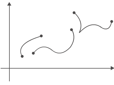
Laplace transform is a method used to go from one domain to another domain. In this case we go from the time domain (t) to the frequency domain (s).
As for most conversions, if there is one way to go from one unit to another, there should be a way to go backwards. It applies in this case also, although it isn’t necessarily a unit. In this case it’s simply called “Inverse Laplace Transform”. In this case we go from the Frequency domain (s), back to the time domain (t).
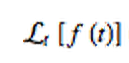
The notation for the Laplace transform is:

The “L” is used to denote Laplace transform. What is inside the curly braces is the function you want to transform from the time domain to the frequency domain.
You may sometimes also see this notation which means the same as the one before:
As for the Laplace transform, it is denoted:
This will give you F(s).
In order to get to the original time domain, you need to take the inverse Laplace transform of F(s) which is:
Now that we got the notation down for the Laplace transform we can go into more depth.
The general formula for the Laplace transform where ‘t’ is greater than or equal to zero:
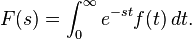 We evaluate at t is greater than or equal to zero because we want to satisfy two conditions:
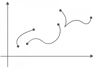
1. The function f(t) has to be piecewise continuous from the interval [0,A]. Simply means a function that is broken apart into different pieces but still continues on. For example:
2. The same function f(t) must be of exponential order. This means that the function f(t) must be smaller than or equal to ke^(at) when t is grater than or equal to M. In this case the variables K, M, and a are just constants and K, M are positive.
As for the inverse Laplace transform, there isn’t any set equation or method of doing it. The way the inverse Laplace transform is denoted, is by the following:
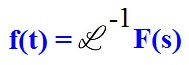
It simply mean to get the function f(t) you would need to take the inverse Laplace transform of F(s).
The main reason we use Laplace transform is because it makes certain (not all) differential equations easier.
A small introduction on the steps to take when solving a Laplace transform problem. There are five steps that we can use to solve a differential equation using Laplace transform:
1. Have a differential equation to solve
2. Take the Laplace transform of both sides in the equation. This will give you a simple algebraic equation to solve.
3. Solve the algebraic equation
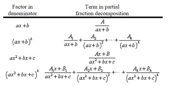
4. Simplify the algebraic so you have what you are solving for on the left side and what it is equal to on the right side. If you can simplify the right side it will make it easier. Once simplified use partial fractions to solve for the unknowns.
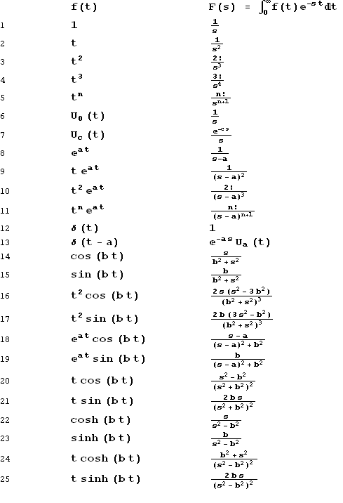
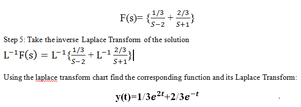
5. Take the inverse Laplace transform and you will have your solution for the differential equation.
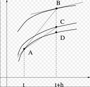
") from the slope of the previous point
from the slope of the previous point ") . This yields the equation
. This yields the equation ") , where the function f represent the slope, or y'(t), and h is the step size. This proves rather inaccurate as the slope at the new point won’t be the same slope of the previous point. In backwards Euler, one considers the same scenario, but takes into account the line connected the two points. Instead of taking the slope at the previous point
, where the function f represent the slope, or y'(t), and h is the step size. This proves rather inaccurate as the slope at the new point won’t be the same slope of the previous point. In backwards Euler, one considers the same scenario, but takes into account the line connected the two points. Instead of taking the slope at the previous point ") , one takes the slope at the new point
, one takes the slope at the new point ") for the backwards Euler method.
for the backwards Euler method.=1, h = .05") approximate y(1)
approximate y(1)")
")
")


")
")
")


")
")
")
")
")
")


,1+0.5(0.5)(-1))")
")


,1+0.5(0.5)(-0.6875))")
")


")
)")
")


+2(-0.765625)+(-0.3671875)}{6})")

")


,0.6438802083+0.5(0.5)(-0.3938802083))")
")


,0.6438802083+0.5(0.5)(0.0170898438))")
")


)")
")


+2(-0.0856526692)+(0.3989461263)}{6})")

=1.31317e^{-4t}\sin(7.31057t)+2.4e^{-4t}\cos(7.31057t)")
=-22.798e^{-4t}\sin(7.31057t)")
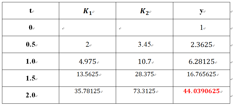
 plus step size h time the previously calculated slope. the general formula is,
%3Dy_n%2Bhf(t_n%2Cy_n)) However, the error for the Euler’s Method depends on the step size. the only way to decrease the error is to reduce the step size, but it will increase the amount of calculations. it only roughly decreases the error by half.
However, the error for the Euler’s Method depends on the step size. the only way to decrease the error is to reduce the step size, but it will increase the amount of calculations. it only roughly decreases the error by half.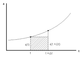
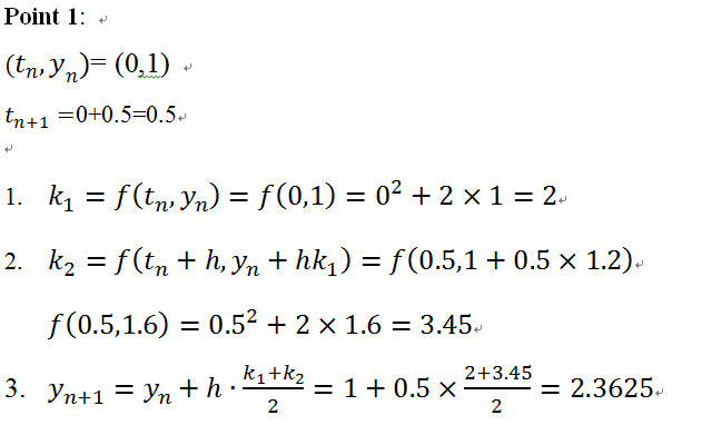
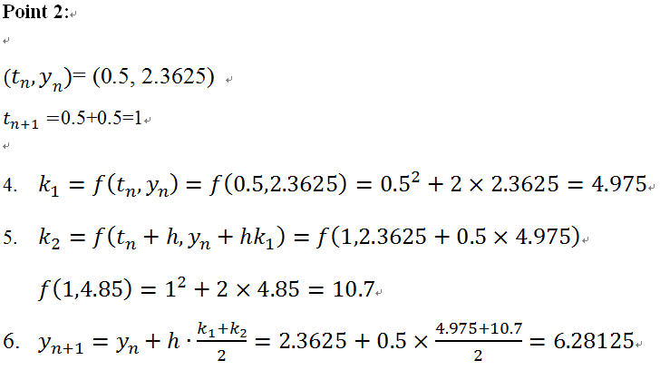
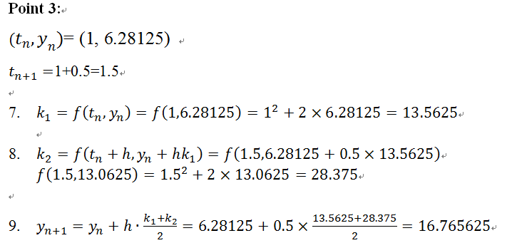
)
)
%3Df(t_n%2Bh%2Cy_n%2Bh((k_1%2Bk_2)%2F2)))
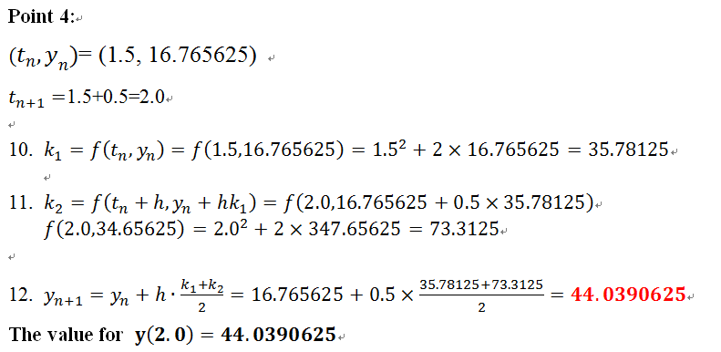
) and
and ) at the beginning of each step because the calculations are all based on these values. This method involved with a lot of calculations, it is recommended after each point, write the values in a table. It will be easy for yourself to look up and check. For each point, the calculations approach to the next new point are the same, so if you set up the three steps, it will be very clear for you to continue to the next step.
at the beginning of each step because the calculations are all based on these values. This method involved with a lot of calculations, it is recommended after each point, write the values in a table. It will be easy for yourself to look up and check. For each point, the calculations approach to the next new point are the same, so if you set up the three steps, it will be very clear for you to continue to the next step.