Monthly Archives: April 2015

Second order linear homogeneous equations with constant coefficients

You have probably seen first order linear equations. Now we”ll move to second order linear equations. What makes it linear? A differential equation is linear if it is a linear function of the variables y, y’, y” and so on.

The standard form of the second order linear equation is

y” + p(t)y’ + q(t)y = g(t)

where p(t), q(t), and g(t) are constant coefficients.
There can also be a constant coefficient in front of the y”.
When g(t) = 0, we can call the differential equation homogeneous, otherwise it is a non-homogeneous.
We can write the second order linear homogeneous equation can be written as:

ay”+by’+cy=0

From that, we can write that characteristic equation:

ar^2+br+c=0

From the characteristic equation, we can find the roots. The roots can come out to be real roots, repeated roots, or complex roots. But we will only focus on real roots.
How do we know if the roots are real roots? We can find out by find out the discriminant. To find out the discriminant, we use b^2-4ac. For the roots to be real, it must follow this condition:

b^2-4ac > 0

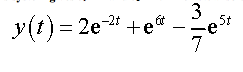
After finding out the roots, we can plug it into the general solution which is:

y(t)=C1e^(r1*t)+C2e^(r2*t)

Now we can figure out the derivative of the general solution which we’ll use later.

y'(t)=(r1)C1e^(r1*t)+(r2)C2e^(r2*t))

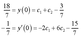
With problems like these, we will have initial condition, y(0) and y'(0), which will be used to find C1 and C2 to determine the particular solution.
You plug in the initial to determine C1 and C2.
Once you determined C1 and C2, plug them back into the general solution to get the particular solution satisfying the initial condition.
The initial conditions gives us a unique solution.
Example 1:      y” + 5y’ + 6y = 0         y(0) = 2     y'(0) = 3
We start out with the characteristic equation which is:

r^2 + 5r + 5 = 0

Now find the roots anyway you feel comfortable with.
One way is by using the quadratic formula.
Now we got

r1 = (-2)
r2 = (-3)

We can plug it into the general solution

y(t)=C1e^(-2t)+C2e^(-3t)

Now that we have to figure out the derivative of general solution which will be:

y'(t)=(-2)C1e^(-2t)-3C2e^(-3t)

Now we can plug in the initial values which are y(0) = 2     y'(0) = 3
For the initial condition y(0) = 2:

2=C1e^(-2*0)+C2e^(-3*0)
2=C1+C2

For the initial condition y'(0) = 3:

3=(-2)C1e^(-2*0)-3C2e^(-3*0)
3=-2C1-3C2

Now that we have 2 equations, we can use them to solve for C1 and C2:

2=C1+C2
3=-2C1-3C2

Multiply the first equation by 2 so the C1 can cancel out.

4=2C1+2C2
3=-2C1-3C2
7=-1C2
C2=(-7)

Now that we know C2, we can plug it back into any of the two equations to find C1.

2=(-7)+C1
C1=9

Lastly we plug the C1 and C2 into the general solution to determine the particular solution.

y(t)=9e^(-2t)-7e^(-3t)

Videos to help with Second order linear homogeneous equations with constant coefficients:
This video is a transition from first order linear differential equations to second order linear differential equations.


This video goes into more detail when the roots are repeated or complex. It only goes up the general solution


In this video, he does a whole example using initial conditions.

Nonhomogeneous Method of Undetermined Coefficients

Nonhomogeneous Method of Undetermined Coefficients

 In this area we will investigate the first technique that can be utilized to locate a specific answer for a nonhomogeneous differential mathematical statement.

Screen Shot 2015-04-30 at 10.15.48 PM  One of the primary points of interest of this strategy is that it diminishes the issue down to a polynomial math issue. The variable based math can get untidy every so often, however for the majority of the issues it won’t be appallingly troublesome. Another decent thing about this system is that the corresponding arrangement won’t be unequivocally needed, albeit as we will see information of the reciprocal arrangement will be required now and again thus we’ll by and large find that also. There are two inconveniences to this system. To begin with, it will work for a genuinely little class of g(t)’s. The class of g(t) for which the technique works, does incorporate a percentage of the more basic capacities, nonetheless, there are numerous capacities out there for which undetermined coefficients just won’t work. Second, it is by and large helpful for consistent coefficient differential mathematical statements.

 The technique is truly straightforward. All that we have to do is take a gander at g(t) and make a speculation as to the type of YP(t) leaving the coefficient(s) undetermined (and thus the name of the system). Plug the conjecture into the differential mathematical statement and check whether we can focus estimations of the coefficients. In the event that we can focus values for the coefficients then we speculated effectively, on the off chance that we can’t discover qualities for the coefficients then we speculated inaccurately.

 let’s jump into example:


Screen Shot 2015-04-30 at 10.15.53 PM                                     

The point here is to find a particular solution, however the first thing that we’re going to do is find the complementary solution to this differential equation.  Recall that the complementary solution comes from solving,                                             

Screen Shot 2015-04-30 at 10.16.03 PMThe characteristic equation for this differential equation and its roots are.

                        Screen Shot 2015-04-30 at 10.16.11 PM

 The complementary solution is then,

                                          Screen Shot 2015-04-30 at 10.16.18 PM

 The technique is truly straightforward. All that we have to do is take a gander at g(t) and make a speculation as to the type of YP(t) leaving the coefficient(s) undetermined (and thus the name of the system). Plug the conjecture into the differential mathematical statement and check whether we can focus estimations of the coefficients. In the event that we can focus values for the coefficients then we speculated effectively, on the off chance that we can’t discover qualities for the coefficients then we speculated inaccurately.

 Presently, how about we continue with discovering a specific arrangement. As said proceeding the begin of this case we have to make a supposition as to the type of a specific answer for this differential mathematical statement. Since g(t) is an exponential and we realize that exponentials never simply show up or vanish in the separation process it appears that a possible type of the specific arrangement would be.

                                                Screen Shot 2015-04-30 at 10.16.26 PM

 Now, all that we need to do is do a couple of derivatives, plug this into the differential equation and see if we can determine what A needs to be. 

 Plugging into the differential equation gives

                                            Screen Shot 2015-04-30 at 10.16.42 PM

 So, in order for our guess to be a solution we will need to choose A so that the coefficients of the exponentials on either side of the equal sign are the same.  In other words we need to choose A so that,

                                                Screen Shot 2015-04-30 at 10.16.49 PM

 Okay, we found a value for the coefficient.  This means that we guessed correctly.  A particular solution to the differential equation is then,

Screen Shot 2015-04-30 at 10.16.57 PM

Before continuing any further we should again take note of that we began off the arrangement above by discovering the corresponding arrangement. This is not actually part the technique for Undetermined Coefficients on the other hand, as we’ll in the long run see, having this under control before we make our supposition for the specific arrangement can spare us a great deal of work and/or migraine. Discovering the corresponding arrangement first is basically a decent propensity to have.


Screen Shot 2015-04-30 at 10.17.05 PM 

We know that the general solution will be of the form,

                            Screen Shot 2015-04-30 at 10.17.13 PM                             

 In this way, we require the general answer for the nonhomogeneous differential comparison. Taking the integral arrangement and the specific arrangement that we found in the past case we get the accompanying for a general arrangement and its derivative.

  Screen Shot 2015-04-30 at 10.17.21 PM

Now, apply the initial conditions to these.

   Screen Shot 2015-04-30 at 10.17.28 PM

Solving this system gives c1 = 2 and c2 = 1.  The actual solution is then.

                     Screen Shot 2015-04-30 at 10.17.34 PM

here are some links from Khan Academy to help clarify the theory:


  • Overview

A linear differential equation is called homogeneous if the following condition is satisfied: If is a solution, so is , where is an arbitrary (non-zero) constant. Note that in order for this condition to hold, each term in a linear differential equation of the dependent variable y must contain y or any derivative of y.

A separable differential equation is any differential equation that we can write in the following form.


Note that in order for a differential equation to be separable all the y‘s in the differential equation must be multiplied by the derivative and all the x‘s in the differential equation must be on the other side of the equal sign. Solving separable differential equation is fairly easy. We first rewrite the differential equation as the following


Then you integrate both sides.

  • Example


Example 2: Solve the equation

This equation is separable, since the variables can be separated:

The integral of the left‐hand side of this last equation is simply

and the integral of the right‐hand side is evaluated using integration by parts:


The solution of the differential equation is therefore


  • Videos


2.1 Linear Equations; Method of Integrating Factors

Theory:

In mathematics, an integrating factor is a function that is chosen to facilitate the solving of a given equation involving differentials. It is commonly used to solve ordinary differential equations, but is also used within multivariable calculus when multiplying through by an integrating factor allows an inexact differential to be made into an exact differential (which can then be integrated to give a scalar field). This is especially useful in thermodynamics where temperature becomes the integrating factor that makes entropy an exact differential.


Consider an ordinary differential equation that we wish to solve to find out how the variable y depends on the variable x. If the equation is first order then the highest derivative involved is a first derivative. If it is also a linear equation then this means that each term can involve y either as the derivative  OR through a single factor of y. Any such linear first order can be re-arranged to give the following standard form:

dy/dx + P(x)y = Q(x); Where P(x) and Q(x) are functions of x, and in some cases may be constants.

A linear first order o.d.e. can be solved using the integrating factor method. After writing the equation in standard form, P(x) can be identified. One then multiplies the equation by the following “integrating factor”:

IF= e^integral (P (x)dx )

This factor is defined so that the equation becomes equivalent to:

d/dx (IF y) = IF Q(x),

Whereby integrating both sides with respect to x, gives:

IF y = Integral (IF Q(x) dx)

Finally, division by the integrating factor (IF) gives y explicitly in terms of x, i.e. gives the solution to the equation.

Here are some Videos of how the problems are solved.

Video 1:

https://www.youtube.com/watch?v=HbCk18VsjHs

Video 2:

https://www.youtube.com/watch?v=RnYzatmp-_s

This is my partner Robert Morels Part of the project:

  • Overview

What is Integrating factor? To sum it all up its bacially a function that is chosen to make easier to solve  a given equation that has differentials included. Its usually used to answer differential equations. At first you may think the procedure is a bit odd but intill you get towards the end is when it can make more sense. examine an usual differential equation that we need to solve to find out how the variable y depends on the variable x. if we notice that the equation happens to be in first order then the highest derivative involved is a first derivative. Note that if its also a linear equation then this means that each term can involve y either as the derivative dy/dx OR through a single factor of y .

  • Example

An integrating factor is a function by which an ordinary differential equation can be multiplied in order to make it integrable. We begin to spot when it can be used. We begin with starting from a standard form of ordinary differential equation.

(dy)/(dx)+f(x)y=q(x),

Once we get our equation we can jot down that f(x) and g(x) are two random functions of x only. When handling equations like this you must know that this form isn’t separable BUT we can join together the two terms on the left side into a single differential by using an integrating factor.

First we compute the integrating factor IF which is given to us by integrating f(x) then expanding the answer:

IF=e^f(x)

Now we defined F(x)=f(x)dx. When we integrate the function f(x) to get F9X) we don’t adda contstant. We are only focus in the function in the integrating factor F(X).

(dF/dx)=f(x)

This translate to the differential of the integrating factor:

(d/dx)e^F(x)=(dF/dx)x(e^F(x))=f(x)e^F(x)

Where we used the chain rule. We begin to multiply both side of the equation:

(e^F(x))(dy/dx)+f(x)e^F(x)y=g(x)e^F(x)

Here is where you may thing its getting pretty odd, but theres a reason for that is that the left hand side is now simply the differential of the integratinf factor multiplied by y:

d/dx(e^F(x)y)=(e^F(x))(dy/dx)+f(x)e^F(x)y

This now gives us a chance to write out the orginal equation in a simpler format:

d/dx(e^F(x)y)=g(x)e^F(x)

now we begin to integrate both sides

d/dx(e^F(x)y)dx=g(x)(e^F(x))dx

Integration is the opposite of differentiation, which makes it possible for the left side to cancel each other out, we then get the following:

e^F(x)y=g(x)(e^F(x))dx

if the integration on the right side is easy to compute this will lead towards our solution.

  • Videos

I included some videos that solve different equations using the method I provided above.

Video # 1:

Video #2:

In this pertectlar video the instructor is solving the following equation of

(dy/dx)+3y=x


Linear Equations; Method of Integrating Factors

1. Overview

What is Integrating factor? To sum it all up its basically a function that is chosen to make easier to solve  a given equation that has differentials included. It’s usually used to answer differential equations.. At first you may think the procedure is a bit odd but until you get towards the end is when it can make more sense. Examine a usual differential equation that we need to solve to find out how the variable y depends on the variable x. if we notice that the equation happens to be in first order then the highest derivative involved is a first derivative. Note that if it’s also a linear equation then this means that each term can involve y either as the derivative dy/dx OR through a single factor of y .

 2. Example

 An integrating factor is a function by which an ordinary differential equation can be multiplied in order to make it integral. We begin to spot when it can be used. We begin with starting from a standard form of ordinary differential equation.

(dy)/(dx)+f(x)y=q(x),

Once we get our equation we can jot down that f(x) and g(x) are two random functions of x only. When handling equations like this you must know that this form isn’t separable BUT we can join together the two terms on the left side into a single differential by using an integrating factor.

First we compute the integrating factor IF which is given to us by integrating f(x) then expanding the answer:

IF=e^f(x)

Now we defined F(x)=f(x)dx. When we integrate the function f(x) to get F9X) we don’t add a constant. We are only focus in the function in the integrating factor F(X).

(dF/dx)=f(x)

This translates to the differential of the integrating factor:

(d/dx)e^F(x)=(dF/dx)x(e^F(x))=f(x)e^F(x)

Where we used the chain rule. We begin to multiply both side of the equation:

(e^F(x))(dy/dx)+f(x)e^F(x)y=g(x)e^F(x)

Here is where you may thing its getting pretty odd, but there’s a reason for that is that the left hand side is now simply the differential of the integrating factor multiplied by y:

d/dx(e^F(x)y)=(e^F(x))(dy/dx)+f(x)e^F(x)y

This now gives us a chance to write out the original equation in a simpler format:

d/dx(e^F(x)y)=g(x)e^F(x)

Now we begin to integrate both sides

d/dx(e^F(x)y)dx=g(x)(e^F(x))dx

Integration is the opposite of differentiation, which makes it possible for the left side to cancel each other out, we then get the following:

e^F(x)y=g(x)(e^F(x))dx

if the integration on the right side is easy to compute this will lead towards our solution.

 3. Videos

 I included some videos that solve different equations using the method I provided above.

Video #2

In this particular video the instructor is solving the following equation of

(dy/dx)+3y=x

-By: Robert Morel

———————————————————————————————–

My Partner Rahman Hasanuzzaman went along to review Linear Equations

Theory:

 In mathematics, an integrating factor is a function that is chosen to facilitate the solving of a given equation involving differentials. It is commonly used to solve ordinary differential equations, but is also used within multivariable calculus when multiplying through by an integrating factor allows an inexact differential to be made into an exact differential (which can then be integrated to give a scalar field). This is especially useful in thermodynamics where temperature becomes the integrating factor that makes entropy an exact differential.

Consider an ordinary differential equation that we wish to solve to find out how the variable y depends on the variable x. If the equation is first order then the highest derivative involved is a first derivative. If it is also a linear equation then this means that each term can involve y either as the derivative  OR through a single factor of y. Any such linear first order can be re-arranged to give the following standard form:

 dy/dx + P(x)y = Q(x);

Where P(x) and Q(x) are functions of x, and in some cases may be constants.

A linear first order o.d.e. can be solved using the integrating factor method. After writing the equation in standard form, P(x) can be identified. One then multiplies the equation by the following “integrating factor”:

 IF= e^integral (P (x)dx )

 This factor is defined so that the equation becomes equivalent to:

 d/dx (IF y) = IF Q(x),

Whereby integrating both sides with respect to x, gives:

IF y = Integral (IF Q(x) dx)


Finally, division by the integrating factor (IF) gives y explicitly in terms of x, i.e. gives the solution to the equation.

Video 1:

Video 2:


Study Guide for Separable Equation

  1. Overview

What are separable equation and how to solve it ?

A differential equation is considered separable if the two variables can be moved to opposite sides of the equation. This facilitates solving a homogenous differential equation, which can be difficult to solve without separation.We are now going to start looking at nonlinear first order differential equations. The first type of nonlinear first order differential equations that we will look at is separable differential equations

A separable differential equation is any differential equation that we can write in the following form.

Note that in order for a differential equation to be separable all the y‘s in the differential equation must be multiplied by the derivative and all the x‘s in the differential equation must be on the other side of the equal sign. Also Consider the equation . This equation can be rearranged to . Any equation that can be manipulated this way is separable. The equation is solved by integrating both sides, resulting in an implicit solution. If an initial condition is provided, you can solve the implicit solution for an explicit solution, and determine the interval of validity, the range of x where the solution is valid. The interval of validity must be continuous and must contain the x-value given in the original condition.

2. Example  

Lets solve a simple question about separable equation.  differential equation: 2(dy)/(dx)=(y(x+1))/(x).                                                                       First of all we have to separate the variables that we have to move all the xs to one side and all the ys to the other. so first step we do is multiply dx on both side so we can cancel the y on the right side so it will give us                              (2dy)=(y(x+1)dx)/(x) and then we divide y on both sides too, so we can cancel the y on the right side. This will give us (2dy)/(y)=(1+1/x)dx  . Now all the y in one side and x is in the other side so we can solve it now by taking the integral on both sides. Therefor

(integral) (2dy)/(y)=integral(1+1/x)dx

So use the answer is 2 ln y= x+ln x+C

3. Video

Here is some videos about separable equation that I copy form KHAN academy if you still confuse about separable equation please watch and I think It will help you a lot.

This is video explain what is separable equation, watch the video for the detail.

In this video, he is explain some example.

Again some example that how to solve the separable equation correctly.

Best of luck on final.


Bernoulli equation

12345Bernoulli Differential Equations

The form of Bernoulli Equations is y’+p(x) y=q(x)y^n, which n is just some real number. As we known that if n=1 or n=0 then after we plug it in to the n of the equation y’+p(x) y=q(x)y^n then we get y’+p(x) y=q(x)y^0 or y’+p(x) y=q(x)y^1. It shows you that it is just the first order linear differential equation that we already known how to solve it. However, if n ≠ 0, 1 then we need to use another method to solve it and it is called the Bernoulli equations. Here are the steps to solve the Bernoulli Differential Equations. In order to solve the Bernoulli Differential Equations as the first order linear differential equation first we need to set a) v=y^(1-n) and after we take the derivative of it we come up with b) v’= (1-n)y^(-n) y’.

We can get y’ alone by dividing by(1-n)y^(-n), and get y’=v’/((1-n) )*y^n. From the original Bernoulli Differential Equations y’+p(x) y=q(x)y^n. We can divided by y^n from the right side of the equation and get y^(-n) *[y]^’+y^(-n)*p(x)*y=q(x). Then we can substitute y’=v’/((1-n) )*y^n in to y’ in this equation y^(-n) 〖*y〗^’+y^(-n)*p(x) y=q(x) and gety^(-n) (v’/((1-n) ))*y^n+y^(1-n)*p(x) y=q(x), so we can cancel y^(-n) and y^n. We multiply (1-n) both side and get the First Order Differential equation v’ + (1-n)*p(x)*v= (1-n) =q(x)

Example:

y’+2y=3*y^(-8)

As we recognize that n≠1 or 0, so we need to use the Bernoulli Equations to transformed into a linear equation.

n=-8
put n=-8 in to the substitution of
v=y^(1-n)
v=y^(9)
we need to get y so, multiply the exponent 1/9 on each side and get
y=v^(1/9), then we take the derivative of it, and it becomes
y’=1/9*v^(-8/9)*(dv/dt)

after we get y’ and y then we can substitute in to the y’+2y=3*y^(-8) to solve for the linear equation

[1/9*v^(-8/9)*(dv/dt)]+[2v^(1/9)]=3(v^(-8/9))

then we multiply 1/9 on both side and divide by v^(-8/9), then we get

[dv/dt]+[18v]=27, and we recognize it is a First Order Linear Differential Equation dy/dx+p(x)y=f(x)
18 is p(x)
µ(t)=e^(∫p(x))
=e^(∫8dx)
=e^(18t)
we multiply e^(18t) of [dv/dt]+[18v]=27 and get
e^(18t)*[dv/dt]+e^(18t)*[18v]=e^(18t)*27
and take the integral on both side to get v alone so we can substitute y

∫d/dt[e^(18t)*v]=∫e^(18t)*27 and get
e^(18t)*v=27e^(18t)+c divide e^(18t) on both side
v=27/18+ce^(-18t)

we known that v=y^(9) from the beginning and plug it back to v

y^(9)=27/18+ce^(-18t), so we can multiply the exponent on both side by (1/9) and get the answer

y(t)=(1.5+ce^(-18t))^(1/9)

Here are the helpful videos that solve the Bernoulli equation step by step.

1.

Part 1

Part 2

2.

Study Guide to Bernoulli Equations

Overview

What are Bernoulli Equations?

Well to put it simply Bernoulli Equations are first order differential equations. What sets Bernoulli Equations apart from other first order differential equations is that they are nonlinear first order differential equation. When we was first introduced to first order differential equations we learned that the standard form  was :

y’ +p(t)y = g(t) ,  y(to) = yo

What separates Bernoulli Equations from other first order equations is that in standard form, it is not equal to some function that is linear but one that has an exact solution. What this means is that their is some power that is raised to the right side of the equation which we shall call n and n cannot be equal to 0 or 1. this is what makes Bernoulli Equations nonlinear. Now we can change the form of a standard first order linear equation into a nonlinear first order equation:

y’ +p(t)y = q(t)y^(n)  y(to)=yo

The above equation is now the standard form for a Bernoulli equation. What we can now understand from this equation is that  p(t) and q(t) are functions that are continuous. Since n is a real number that has to be n> 0 and n>1 for this  to be non linear.

Now the question is how do we solve Bernoulli Equations?

Sample Problem:

take an equation such as t^(2)y’ + 2ty – y^(3) = 0

and change it by adding y^(3) on both sides and we get:

t^(2)y’ + 2ty = y^(3)

Next we divide by t^(2) to on both sides of the equation so we can get it into standard form.

y’ + 2/yt = y^(3)/t^(2)       <————-STANDARD FORM

Now we can go into the steps to solve this equation;

1. Divide by y^(n)

y’/y^(3) + 2/yt/y^(3) =  (y^(3)/t^(2))/y^(3)

we get: (y’ + 2/yt)/y^(3) = 1/t^(2)

2. We substitute v = y^(1-n)

Since y^(3)

we get:v = y^(1-3) = y^(-2)

now we can rearrange the formula to so we can substitute v into it by moving the y^(2) to the numerator and we get:

y’/y^(3) + 2y^(-2)/t = 1/t^(2)

y’/y^(3) + 2v/t = 1/t^(2) <——————-Substitute v for y^(2)

Before we move to the solve Step we need to take the Derivative of the substitution v = y^(-2)

d/dy y^(-2)

dv/dt = -2y^(-3) dy/dt

(-1/2)v’ = -2y’/y^(3)(-1/2)

Now we can substitute for y’/y^(3) with the above equations and we get:

(-1/2)v’ + (2/t)v = 1/t^(2) <—————– First order linear equation

next we use the method of intergrating factor which states

mu = e^ intergral of (-4/t) which is equal to 1/t^(4)

we then multiply both sides b\by Mu and get the equation:

(dv(t)/dt)/t^(4) + d/dt(1/t^(4))v = (-2/t^(6))

Next we intergrate both sides and we come to the final answer of

y(t) = +- Sqrt(5t)/sqrt(ct^(5) + 2)

Videos:


I \\


Electrical Circuits

Electric circuits can consist of a wide variety of complex components. These may be set up in series, or in parallel, or even as combinations of both. However, we’ll be considering only series circuits with especially simple components: resistors, inductors, and capacitors, along with some form of voltage supply.

To start with, let’s consider the picture of a simple series circuit in which one of each of the components that we mentioned above appears:

electrical circuit


  • L is a constant representing inductance, and is measured in Henry
  • R is a constant representing resistance, and is measured in ohms
  • C is a constant representing capacitance, and is measured in farads
  • E represents the electromotive force, and is measured in volts. It is not necessarily a constant, and may be a function of time

Let Q(t) be the charge in the capacitor at time t (Coulombs). Then dT /dt is called the current, denoted I. The battery produces a voltage (potential difference) resulting in current I when the switch is closed. The resistance R results in a voltage drop of RI. The coil of wire (inductor) produces a magnetic field resisting change in the current. The voltage drop created is L(dI/dt). The capacitor produces a voltage drop of Q/C. Unless R is too large, the capacitor will create sine and cosine solutions and, thus, an alternating flow of current. Kirchhoff Law states that “The sum of the voltage drops across each component in a circuit is equal to the voltage, E, impressed upon the circuit.” so

Restating Kirchhoff’s second law in abbreviated form, we get the following:

sum of the voltage drops = E,

which may be restated as:

inductor voltage drop + resistor voltage drop + capacitor voltage drop = E,

into which we may substitute the actual voltage drops that we mentioned above, to get:

(1) LI′ + RI + q/C = E.

But, also according to physics, I = q′, so substituting, we can rewrite the equation purely in terms of the charge, q, rather than a mixture of charge and current:

(2) Lq″ + Rq′ + q/C = E,

or alternatively, if we differentiate equation (1) and use the same substitution, we get an equation purely in terms of current:

(3) L I″ + R I′ + I/C = E′.

We will be mainly concerned with using the last of these three equivalent forms.

Notice that equation (3) is linear with constant coefficients, so in this case when
E′ = 0, (the homogeneous case), it may be solved very easily, even by hand.

The form of E′ will determine the method necessary when solving the non-homogeneous case by hand. We would need to use either undetermined coefficients, or variation of parameters.

An Example:

E(t) = 2e^t, R= 5Ω, C= 1/6 F, L= 1H


E(t)= Q`R + Q/R + Q/C + LQ“

=> 2e^t = Q`*5 + Q/(1/6) + L*Q“

=>2e^t = Q“ +5Q` + 6Q


r2 + 5r + 6 = 0

r2 + 3r + 2r + 6 =0

(r+3)(r+2) = 0

r = -3

r = -2

Q = Ae-3t + Be-2t

Guess:

Q = Ce^t

Q` = Ce^t

Q“ = Ce^t


Ce^t  + 5Ce^t + 6 Ce^t = 2 e^t

12Ce^t  = 2e^t

6Ce^t = e^t

C = 1/6

Q = Ae^(-3t) + Be^(-2t) + (1/6)e^t

Initial charge Q(0) = 11C

Initial Current I(0) = -18A


Take Q` and plug in

Q = Ae^(-3t) + Be^(-2t) + (1/6)e^t

Here are some videos which may also help to solve electrical Circuit in Differential Equation


Solving Repeated Roots

Once you know how to solve second order linear homogeneous differential equations with constant coefficients, real or complex, the next step is to solve with those that have repeated roots. When solving for repeated roots, you could either factor the polynomial or use the quadratic equation, if the solution has a repeated root it means that the two solutions for “x” or whatever variable are the same.

Theorem for Solving Repeated Roots

Let:   ay” + by’ + cy = 0

Be a differential equation such that the characterstic equation has the repeated root “r” That is :

(b^2)-4ac = 0

Then the general solution to the differential equation is given by

y  =  c1ert + c2tert