Category Archives: Uncategorized

Taylor Series

Posted on May 22, 2015 by Jacob Ramroop | Leave a comment

Taylor Series are very useful for approximating function values, much more effectively than standard linear approximations.

To me Taylor Series is very easy and straight forward. There is one important thing you need to remember about Taylor series and that is
y= a0 + a1x + a2x^(2) + a3x^(3) + a4x^(4)……….+anx^(n)
y’=a1 + 2A2x +3a3x^(2) +4a4x^(3)………..
y”=2a2 + 6a3x + 12a4x^(2)…………………
and with this all you do is plug it into a the equation.
For example
y”+2y’ +y=0 y(0)=0 y’(0)=2 x=1
the first step is to find y, y’, y” which are the given above from earlier. These do not change.
Then you plug it in the formula producing
(2a2 + 6a3x + 12a4x^(2))+ 2(a1 + 2A2x +3a3x^(2) +4a4x^(3)) + (a0 + a1x + a2x^(2) + a3x^(3) + a4x^(4)) …..= 0
(2a2 + 6a3x + 12a4x^(2))+ 2a1 + 4a2x +6a3x^(2) +8a4x^(3) + (a0 + a1x + a2x^(2) + a3x^(3) + a4x^(4)) ……= 0
Now you group by the power of x.
(2a2 + 2a1 + a0) + (6a3x + 4a2x + a1x) + (12a4x^(2) + 6a3x^(2) + a2x^(2) ) + a3x^(3) + a4x^(4))….. = 0
(2a2 + 2a1 + a0) + (6a3 + 4a2 + a1)X + (12a4 + 6a3 + a2 ) x^(2) + a3x^(3) + a4x^(4))….. = 0
Now we set to equal 0
2a2 + 2a1 + a0 =0
6a3 + 4a2 + a1 = 0
12a4 + 6a3 + a2 = 0

Remember y (0) =0 and y’(0)=2
Y(0) = 0 = a0
Y’(0)= 2 = a1
Now knowing that we will plug in a0 and a1
2a2 + 2(2) + 0 =0
2a2 + 4 =0 2a2 =-4 a2 =-2

6a3 + 4(-2) + (2) = 0
6a3 -6 = 0 a3=1
12a4 + 6a3 + a2 = 0
12a4 + 6(1) + (2) = 0
12a4 + 8 = 0 a4= -(1/3)
Now you substitute a0 , a1, a2, a3, and a4 into the first equation.(note we are only doing up to the 5th term if the problem wants up to the 6th term you would find up to a5 )
y= a0 + a1x + a2x^(2) + a3x^(3) + a4x^(4)……….+anx^(n)
Producing
y= 0+ 2x – 2x^(2) + 1x^(3) – (1/3)x^(4)……….+anx^(n)
Then you plug in x in this case x = 1
y(2)= 0+ 2(1) – 2(1)^(2) + 1(1)^(3) – (1/3)(1)^(4)
y(2)= 0+ 2 – 2+ 1 – (1/3)
y(2)= – (2/3)

Laplace Transform: Solution of the Initial Value Problems (Inverse Transform)

Posted on May 20, 2015 by Aayush | 1 comment

The Laplace transform is an important technique in differential equations, and it is also widely used a lot in electrical engineering to solving linear differential equation The Laplace transform takes a function whose domain is in time and transforms it into a function of complex frequency.

The inverse Laplace transform does exactly the opposite, it takes a function whose domain is in complex frequency and gives a function defined in the time domain.

The steps to using the Laplace and inverse Laplace transform with an initial value are as follows:

1) We need to know the transformations we have to apply, which are:

L{y’}=sY(s)-y(0) L{y”}=s^2 Y(s)-sy(0)-y'(0)

2) Once we apply the proper Laplace transform to our function we then apply the initial condition

3)Then since we can’t find y(t) directly, we solve for Y(s), which is the Laplace transform of y(t)

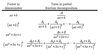
4) Once we find Y(s), we may need to break up the equation into partial fraction form depending on the denominator. there must only be a single term in the denominator and no “s” in the numerator. (look at “Factor in Denominator” chart image attached)

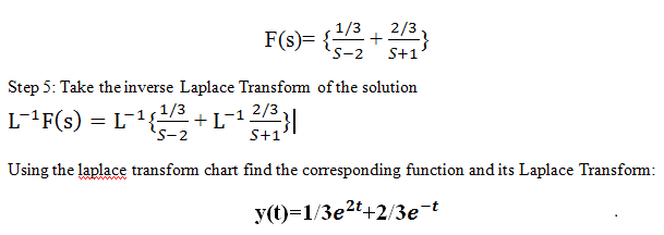
5) We take the inverse Laplace transform to get y(t)

So now to apply those steps,

Let’s take for example, 2y’-y = 1 ; y(0) = 0

1) Apply the transforms. 2(sY(s)-y(0))-Y(s)= 1/s

2) Apply the initial conditions given. 2(sY(s)-0)-Y(s)= 1/s

3) Solve for Y(s). Y(s)(2s-1) = 1/s Y(s)=1/s(2s-1)

4) Apply the inverse transform. L^(-1){1/s(2s-1)} = L^(-1){1/(2s-1)-(1/s)} = e^(1/2t)-1

For another example, let’s take something that requires us to use partial fractions to get the right denominator.

F(s) = [19/(s+2)]-[1/(3s-5)]+[7/(s^5)]

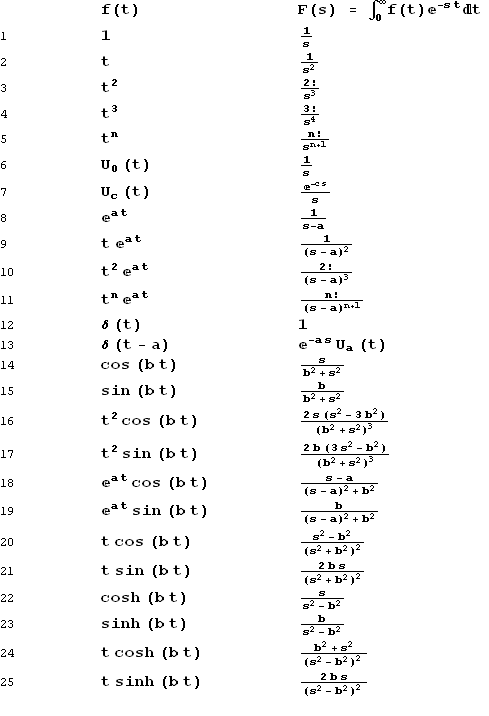
So to get started on this one, we look at the Laplace transform table and see which fraction refers to the transformation. The first fraction looks like 1/(s-a) = e^(at). Although the “a” in this case would be a -2. For the second fraction, we got the same case except that the s is 3s, so all we have to do is factor out the 3, and apply the Laplace transform. And for the third fraction we see that it looks like, (n!)/s^(n+1) = t^n ; and since the exponent in the denominator is 5, the value for n = 4. But now we still have a 7 in the numerator whereas we need a 4! or 24. So to fix this all we have to do is multiply the top numerator by a constant to achieve the desired numerator, but we have to remember to divide by the same constant after taking the Laplace transform.

So it would be:

F(s) = [19/(s-(-2))]-[1/3(s-(5/3))]+[7(4!/4!)/(s^(4+1))]

So, now we have to take the inverse Laplace transform.

f(s) = 19e^(-2t) – (1/3)e^(5t/3) + 7/24(t^4)

I hope that the link to the video and images are helpful.

https://www.khanacademy.org/math/differential-equations/laplace-transform/laplace-transform-to-solve-differential-equation/v/laplace-transform-to-solve-an-equation

1 Comment

Posted in Uncategorized

Tagged Inverse, inverse Laplace, Laplace, Partial fraction, Transform

Improvements on the Euler Method (backwards Euler and Runge-Kutta)

Posted on May 18, 2015 by Daniel Wong | 1 comment

Several improvements to Euler’s Method exist: the backwards Euler method and the Runge-Kutta method (for Improved Euler method see BingJing Zheng’s post Improved Euler’s Method).

Backwards Euler Method with Example

Recalling that in Euler’s method, one approximates the point $(t_{n+1}, y_{n+1})$ from the slope of the previous point $(t_{n},y_{n})$ . This yields the equation $y_{n+1}=y_{n}+hf(t,y)$ , where the function f represent the slope, or y'(t), and h is the step size. This proves rather inaccurate as the slope at the new point won’t be the same slope of the previous point. In backwards Euler, one considers the same scenario, but takes into account the line connected the two points. Instead of taking the slope at the previous point $(t_{n}, y_{n})$ , one takes the slope at the new point $(t_{n+1}, y_{n+1})$ . This yields the equation $y_{n+1}=y_{n}+hf(t_{n+1}, y_{n+1})$ for the backwards Euler method.

Example: Given $y' = t^2-y, y(0)=1, h = .05$ approximate y(1)

Find y at t = 0

Given: At t = 0, y = 1

Find y at t = 0.5

At t = 0.5, $y_{n+1}=y_{n}+h*f(t_{n+1},y_{n+1})$

At t = 0.5, $y_{n+1}=1+0.5y'(0.5,y_{n+1})$

At t = 0.5, $y_{n+1}=1+0.5(0.5^2-y_{n+1})$

At t = 0.5, $1.5y_{n+1}=1.125$

At t = 0.5, $y_{n+1}=0.75$

Find y at t = 1

At t = 1, $y_{n+1}=y_{n}+hf(t_{n+1},y_{n+1})$

At t = 1, $y_{n+1}=0.75+0.5y'(1,y_{n+1})$

At t = 1, $y_{n+1}=0.75+0.5(1^2-y_{n+1})$

At t = 1, $1.5y_{n+1}=1.25$

At t = 1, $y_{n+1}=0.8333333333$

Runge-Kutta Method with Example

Much like the Improved Euler method, one tries to find a better fit for the definite integral of a curve. One uses the idea that a parabola would cover the most area under a curve (compared to a rectangle or trapezoid of other methods). From this idea, one found equations for the following points:

$y_{n+1}=y_{n}+h(\frac{k_{1}+2k_{2}+2k_{3}+k_{4}}{6})$

where

$k_{1}=f(t_{n},y_{n})$

$k_{2}=f(t_{n}+0.5h,y_{n}+0.5hk_{1})$

$k_{3}=f(t_{n}+0.5h,y_{n}+0.5hk_{2})$

$k_{4}=f(t_{n}+h,y_{n}+hk_{3})$

Example: Given $y' = t^2-y, y(0)=1, h = .05$ approximate y(1)

Find y at t = 0

Given: At t = 0, y = 1

Find y at t = 0.5

$k_{1}=f(t_{n},y_{n})$

$k_{1}=y'(0,1)$

$k_{1}=0^2-1$

$k_{1}=-1$

$k_{2}=f(t_{n}+0.5h,y_{n}+0.5hk_{1})$

$k_{2}=y'(0+0.5(0.5),1+0.5(0.5)(-1))$

$k_{2}=y'(0.25,0.75)$

$k_{2}=0.25^2-0.75$

$k_{2}=-0.6875$

$k_{3}=f(t_{n}+0.5h,y_{n}+0.5hk_{2})$

$k_{3}=y'(0+0.5(0.5),1+0.5(0.5)(-0.6875))$

$k_{3}=y'(0.25,0.828125)$

$k_{3}=0.25^2-0.828125$

$k_{3}=-0.765625$

$k_{4}=f(t_{n}+h,y_{n}+h*k_{3})$

$k_{4}=y'(0+0.5,1+0.5(-0.765625))$

$k_{4}=y'(0.5,0.6171875)$

$k_{4}=0.5^2-0.6171875$

$k_{4}=-0.3671875$

$y_{n+1}=y_{n}+h(\frac{k_{1}+2k_{2}+2k_{3}+k_{4}}{6})$

$y_{0.5}=1+0.5(\frac{-1+2(-0.6875)+2(-0.765625)+(-0.3671875)}{6})$

$y_{0.5}=0.6438802083$

Find y at t = 1

$k_{1}=f(t_{n},y_{n})$

$k_{1}=y'(0.5,0.6438802083)$

$k_{1}=0.5^2-0.6438802083$

$k_{1}=-0.3938802083$

$k_{2}=f(t_{n}+0.5h,y_{n}+0.5hk_{1})$

$k_{2}=y'(0.5+0.5(0.5),0.6438802083+0.5(0.5)(-0.3938802083))$

$k_{2}=y'(0.75,0.5454101562)$

$k_{2}=0.75^2-0.5454101562$

$k_{2}=0.0170898438$

$k_{3}=f(t_{n}+0.5h,y_{n}+0.5hk_{2})$

$k_{3}=y'(0.5+0.5(0.5),0.6438802083+0.5(0.5)(0.0170898438))$

$k_{3}=y'(0.75,0.6481526692)$

$k_{3}=0.75^2-0.6481526692$

$k_{3}=-0.0856526692$

$k_{4}=f(t_{n}+h,y_{n}+h*k_{3})$

$k_{4}=y'(0.5+0.5,0.6438802083+0.5(-0.0856526692))$

$k_{4}=y'(1,0.6010538737)$

$k_{4}=1^2-0.6010538737$

$k_{4}=0.3989461263$

$y_{n+1}=y_{n}+h(\frac{k_{1}+2k_{2}+2k_{3}+k_{4}}{6})$

$y_{1}=0.6438802083+0.5(\frac{-0.3938802083+2(0.0170898438)+2(-0.0856526692)+(0.3989461263)}{6})$

$y_{1}=0.6328751629$

Analysis

After answering the same question using both the backwards Euler method and Runge-Kutta method, one can see the accuracy of the results.

The exact solution for y(1) is 0.6321205588.

Using the Euler method, y(1) is approximately 0.375.

Using the backwards Euler method, y(1) is approximately 0.8333333333.

Using the Runge-Kutta method, y(1) is approximately 0.6328751629.

The backwards Euler method provides a better approximation than the Euler method, with a few more steps. The Runge-Kutta method provides the best approximation, but involves more calculation.

1 Comment

Posted in Uncategorized

Tagged Backwards Euler Method, Improvement on the Euler Method, Runge-Kutta Method

Posted on May 17, 2015 by Vanessa Mejia | 2 comments

6.2 Laplace Transform: Solution of the Initial Value Problems (Inverse Transform)

Laplace transform is used to convert a function in the t domain and transfer it to the s domain. The practical used of this transform is to solve differential equations easier. Having read the definitions and having knowledge on how the Laplace transform works we would proceed with an example in how to apply it to a differential equation with initial values.

1.Solve using Laplace Transform

y”-y’-2y=0 with the condition y(0)=1 y’=0

Step 1: Step 1 is it a differential equation? Yes, because its homogeneous and linear

Step 2: Take the Laplace from both sides L{ y”-y’-2y=0}

Step 3:Solve it algebraically

using the laplace transform chart we know f”(t)= L{f(t)-sf(0)-f'(0)

f'(t)=sL{f(t)-f(0)

Take the Laplace of the diff equation applied the initial value given :

Y(s)-s(1)-0-{sY(s)-1}-2Y(s)

Factor Y(s): Y(s)(-s-2)-s+1=0

Isolate the Y(s) : Y(s)=

therefore take -s+1 to the other side and divide from the quadric equation

Step 4: Simplify the solution by applying partial fraction

= +

= (s-2)(s+1)=A(s+1) = (s-2)(s+1)=B(s-2)

s-1= A(s+1)+B(s-2)

“”= As+A+Bs-2B

“”= As+Bs+A-2B

Combine all the letter that have s with s, and number with the terms that don’t have s on it.

A+B=1 since (1) is in front of the s we use 1 -1=A-2B

Solve the linear equations : we would solve this by using elimination method:

A-2B= -1

2A+2B=2

3A=1 therefore, A=1/3 then by substituting A into the A+B=1– (1/3)+B=1

we obtain B=2/3 and A=1/3

Finally your function is in s domain:

Reminder outline to solving differential equation using Laplace transform:

1. Start with a differential equation

Take the Laplace Transform from both side of the equation
Then you would have to simplify the algebraic solution.
This would require a method like partial fraction

4.Take the inverse Laplace transform of the solution, this would be your solution for the differential equation, at this point you should be in the t domain with a simplify equation

Important Notation:

L{f(t)}: The “L” is used to note that the function {f(t)} laplace transform is being applied.

F(s) : When working with Laplace Transform anything noted with a capital means you are working in s domain. Therefore, F(s) means the function f(t) is already transfer in the s domain.

{F(S)}: is used when working on the inverse laplace transform therefore going back to your function in the t domain.

2 Comments

Posted in Uncategorized

Series Solutions around an ordinary point…. Taylor Series : Sec 5.2

Posted on May 17, 2015 by kumar Pryce | 2 comments

Overview
We are considering methods of solving second order linear equations when the coefficients are functions of the independent variable. We consider the second order linear homogeneous equation
P(x) d2 y/ dx2 + Q(x) dy/ dx + R(x)y = 0 (equation 1)
Since the procedure for the non-homogeneous equation is similar. Many problems in mathematical physics lead to equations of this form having polynomial coefficients; examples include the Bessel equation
X2 y’’ + xy’ + (x2 – a 22) y = 0
Where (a) is a constant, and the Legendre equation
(1 – x 2 ) y’’ – 2xy’ + c(c + 1) y = 0 Where (c) is a constant
Given the equation
P(x) d2 y/ dx2 + Q(x) dy /dx + R(x)y = 0
The equation
d2 y/ dx2 + Q(x) P(x) dy/ dx + R(x) P(x) y = 0 or d2 y/ dx2 + p(x) dy/ dx + q(x)y = 0
Where p(x) = Q(x)/ P(x) and q(x) = R(x) /P(x)
is called the equivalent normalized form of equation. The point (a) is called an ordinary point of equation (1). That is to say that these two quantities have Taylor series around x=x0. We are going to be only dealing with coefficients that are polynomials so this will be equivalent to saying that

for most of the problems. The basic idea to finding a series solution to a differential equation is to assume that we can write the solution as a power series in the form,
Y(x)= ∑_(n=0)^∞▒〖An (x-Xo)^n〗

and then try to determine what the an’s need to be. We will only be able to do this if the point x=x0, is an ordinary point. We will usually say that is a series solution around x=x0.

Example

y”+y=0

Suppose that has a Taylor series about x=0

y(x) = xⁿ= a₀+a₁x+a₂x²+a₃x³+a₄x⁴

Substitute into the differential equation and simplify by grouping together terms with similar powers of

We start with the assumption that

Y(x) = a₀+a₁x+a₂x²+a₃x³+a₄x⁴+ …..

Y’(x) = a₁+2a₂x+3a₃x²+4a₄x³+……

Y”(x) = 2a₂+6a₃x+12a₄x²+……

Now substitute and into the differential equation

Y’’+y= 0:

(2a₂+6a₃x+12a₄x²+……) +( a₀+a₁x+a₂x²+a₃x³+a₄x⁴+ …..) = 0

Get rid of parentheses (don’t forget to distribute the and the in front of the second and third sets of parentheses

2a₂+6a₃x+12a₄x²+…+ a₀+a₁x+a₂x²+a₃x³+a₄x⁴+ ….= 0

Now group together by powers of :

(2a₂₊a₀)+ (6a₃+a₁)x +(12a₄+a₂)x²+(20a₅+a₃)x³+…= 0

Finally, we compare each term on the left with the corresponding term on the right – since the right side is zero, each of the expressions in the parentheses (which give the coefficients of the powers of ) must also be equal to zero:

2a₂+a₀=0
6a₃+a₁=0
12a4+a2=0
20a₅+a₃=0
……

Then you find the first 5 terms ( coefficients)

a₀=0
a₁=0
a₂= a₀/2
a₃= a₁/6
a₄= a₀/ 24

This gives us the coefficients to determine the first five terms of the Taylor Series, Remembering that Y(x) = a₀+a₁x+a₂x²+a₃x³+a₄x⁴+…. we substitute in the values of to obtain

Y=a₀+a₁x+a₀/2 x²+a₁/6 x³+ a₀/24 x⁴

3. In case I wasn’t clear enough with the explanation or steps needed to solve the equation i will add a couple of video hopefully they help.

2 Comments

Posted in Uncategorized

Laplace Definition “Study Guide”

Posted on May 7, 2015 by abraham | 3 comments

Laplace transformation “transform” a differential equation into an algebraic equation by changing the equation from the time domain to the frequency domain. The differential equation is packed into one or more Laplace transform equivalent forms and manipulated algebraically.

If we apply the Laplace transformation correctly we can save a lot of time and effort. Even when the complexity of the operation required are reduced significantly, it is necessary to pay attention to the parameter contained in the Laplace transformation table.

The following equation to convert an equation from the time domain to the frequency domain:

To avoid having to do this process every single time a transform table has been created. This table can be used to convert f(t) into its F(s) equivalent and can be used to bring F(s) back into f(t). The transform table has some important parameter such as the values for “s” that are valid for that specific equation. This is the domain of convergence for that equation and is very important to understand it in order to apply the Laplace transform correctly.

Importance of the “s” value: “s>0” and “s>a”

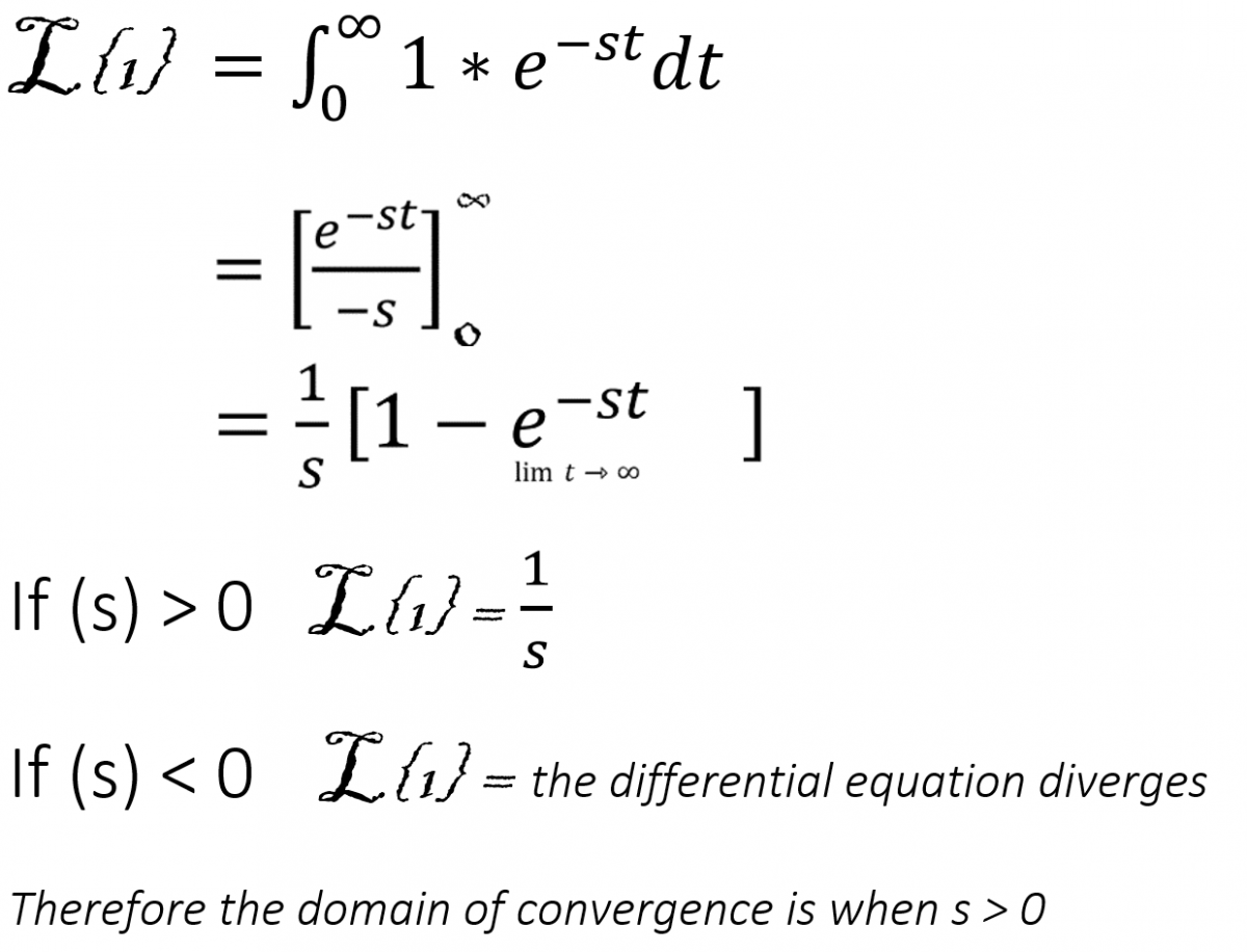
In the following example we can see the reason for the restriction: “s > 0”. When we evaluate the integral for “s > 0” the integral converges to 1/s, but when we plug-in zero, the integral diverges and we have no solution for the integral.

Let’s take the Laplace of 1:

Fitting the equation into the Laplace transform table:

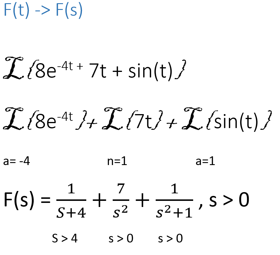
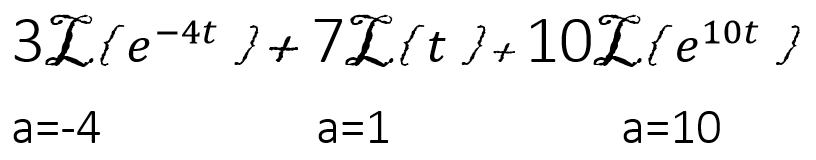
Sometimes the given equations doesn’t seem to fit any of the forms in the transform table. To solve this problem we have to use algebraic techniques to brake the equation into parts that fit the transform table. For example:

Laplace transform in 5 steps:

1. Start with a differential equation.

The first steps is have a differential equation f (t).

2. Take Laplace transformation of both sides.

The transformation has to be taken entirely on both sides of the differential
equation. Sometimes the differential equation doesn’t match the transform table
and we have to use algebraic techniques to force it to match. For example:

separate the parts of the equation connected by addition or subtraction,
to match the table, find the values for a and/or be as required by the table:

Make sure you input the “a” value correctly (check for the sign)
state the values for convergence. In this case “s > 0” since all
individual pieces of the equation converge when “s> 0”

3. Solve the resulting equation.

Once we have the equation in the frequency domain we can solve for
Laplace of y: L {y}

4. Simplify the solution.

Once we found L {y} we will proceed to reverse process done
in part 2, to match the transform table we might need to use
partial fractions or other algebraic techniques to separate the
Solution into parts that match the table.
As in step 2 watch carefully for the values of “a “and/or “s”

Example:

5. Take the inverse Laplace.

Once the solution is simplified we take inverse Laplace to bring
the equation back to time domain.

a pdf copy of this document available here: Laplace transformation

3 Comments

Posted in Uncategorized

Exam 3 Review – CORRECTIONS

Posted on May 6, 2015 by Jonas Reitz | 1 comment

Hi everyone,

I’ve updated the answer to Problem 1b on the Exam #3 Review. It should be:

1b. $I(t)=-234.261e^{-15t}\sin(32.0156t)$

NOTE: The term involving cosine disappears because the coefficient turns out to be zero – although, based on the number of decimals you used, you may have a number very close to zero instead (rounding error).

Regards,
Prof. Reitz

1 Comment

Posted in Uncategorized

Tagged corrections, exam 3 review

Euler’s Method

Posted on May 4, 2015 by d.Santos | 1 comment

When given a first order differential equation, we may use the various types of strategies that we earned such as exact, linear, separable, etc. Sometimes these strategies do not help us solve the equation meaning we can’t find an explicit solution (can’t find y=…). This is where Euler’s method comes into play. Euler’s method helps us find an approximation for the solution of a differential equation by generating a series of points. . The foundation for Euler’s Method is to use the concept of local linearity to join the multiple small line segments so that they make a close approximation to the function.

Definition of local linearity: if you zoom in (using the same zoom factor in both directions) on a point on the graph, the graph eventually appears to be a straight line whose slope is the same as the slope (derivative) of the tangent line at that point.

Euler’s Method Formula: y_n+1=y_n + h*f(t_n,y_n)

For Euler’s Method we are given useful information (“givens”) to help us find y_n. The givens are:

The differential equation y’= f(t_n,y_n)

NOTE: This helps us find the slope for the points by plugging in the points into the equation.

Initial value point y(t₀)=y₀, also written as (t_0,y_o)

NOTE: We use our initial value to find

(t_1,y₁)

(t_2,y₂)

(t_3,y₃)

(t_n,y_n)

The step size h. (optional)

NOTE: When the step size is not given, it is up to your discretion to decide whether you want a close approximation or not. Recall, in Calculus I, we learned how to find the area under the curve. The basic idea is to use smaller rectangles under that curve, so our area approximation can be close as possible to the actual area. This idea is the same for the step size, the smaller your step size is from one point to the other, the closer your approximation for the point y(t_n)= y_nwill be. Also, because of the step size we are allowed to find the values of the succeeding t’s by adding the step size to the preceding t.

Sample Problem:

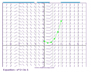
Given y’= t²+3t-1, y(0)=1. Find the value of y(2).

Step 1:

We have to decide on the step size (h) to find the next series of points until we get to y(2) . A good guess for an approximation may be 0.5. It depends on how many steps you would like to use. Let’s say I want to use 5 steps. A formula to let me know what my value of h will be:

where n= the steps that will be used. Let’s plug it in and see if the guess will give me a better approximation

Screen Shot 2015-05-04 at 11.10.31 AM

So, we were off by 0.1. We will use 0.4.

Step 2: Find the “t”s

We use our step size and add on to the previous t

t₁= t_o + 0.4 = 0 + 0.4 = 0.4

t₂= t₁ + 0.4 = 0.4 + 0.4 = 0.8

t₃= t₂ + 0.4 = 0.8 + 0.4 = 1.2

t₄= t₃ + 0.4 = 1.2 + 0.4 = 1.6

t₅= t₄ + 0.4 = 1.6 + 0.4 = 2

NOTE: Last Step size should be the value that are ask to find, y(2)

Step 3: Finding our slopes to find our “y”s. We use the Euler’s Method formula to find our slope first, in order to find the succeeding y. It’s like recursive sequences, we cannot proceed to the next points without the preceding data from the previous equation.

y_n+1=y_n + h*f(t_n,y_n)

What we know:

Previous “y”s
How to find the slope
h=0.4

y₁=y₀+ 0.4 x ((0)²+3(0)-1)= 1+0.4(-1)=0.6

y₂=y₁+ 0.4 x ((0.4)²+3(0.4)-1)= 0.6+0.4(0.36)=0.744

y₃=y₂+ 0.4 x ((0.8)²+3(0.8)-1)= 0.744+0.4(2.04)=1.56

y₄=y₃+ 0.4 x ((1.2)²+3(1.2)-1)= 1.56+0.4(4.04)=3.176

y₅=y₄+ 0.4 x ((1.6)²+3(1.6)-1)= 3.176+0.4(6.36)=5.72

A table is also helpful when finding the solution.

Subscript	t	y	y’
0	0	1	(0)²+3(0)-1=-1
1	0.4	0.6	(0.4)²+3(0.4)-1
2	0.8	0.744	(0.8)²+3(0.8)-1
3	1.2	1.56	(1.2)²+3(1.2)-1
4	1.6	3.176	(1.6)²+3(1.6)-1
5	2	5.72	(2)²+3(2)-1

Screen Shot 2015-05-04 at 11.15.04 AM

Note: You can also see a visual of Euler’s Method (graphically) using graphic software. The graph below is from www.mathscoop.com

Screen Shot 2015-05-04 at 11.16.35 AM

Here is another great example:

1 Comment

Posted in Uncategorized

Repeated Roots Second Order Linear Homogeneous Equation

Posted on May 1, 2015 by Carolina | 4 comments

Overview

Second order linear equations become homogeneous when the linear function of y and y’ (which can be written in the form y” + p(t)y’ + q(t)y = g(t)) is equal to zero. In other words when g(t)=0.

This guide will be discussing how to solve homogeneous linear second order differential equation with constant coefficient, which is written in the following form:

y”+by’+cy = 0

The first step is to use the equation above to turn the differential equation into a characteristic equation. The characteristic equation is written in the following form:

r² +br+c = 0

Second to find the roots, or r₁and r₂you can either factor or use the quadratic formula:

r² = ± -b √b²-4ac

It is important to remember when to the particular equation above. There will problems where the variable a is not needed in the quadratic formula because there will be no a in the differential equation. In the cases where there is no a variable limit the a variable from the quadratic equation. The quadratic equation will the look like the following:

r² = ± -b √b²-4c

Once you get repeated roots , or r₁ and r₂ from the characteristic equation then y = e^rt is considered a solution of the differential equation.

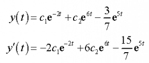
The next step would be to plug r₁ and r₂ into the general equation:

y = C₁ e^r1t +C₂ e^r2t

Another important thing to realize and remember is that when solving a homogeneous equation for a repeated root the solution will end up cancelling out. In order to avoid this a “t” needs to be place in the general solution. The general solution for the repeated root will then be in the following form:

y = C₁ e^r1t +C₂t e^r2t

Sample Problem

Problem 1:

y”+12y’+36 = 0

Step 1: Turn the differential equation into a characteristic equation

r² + br + c = 0

r² + 12r + 36 = 0

Step 2: Factor the characteristic equation

r² + 12r + 36 = 0

(r + 6) (r + 6) = 0

r₁ = -6 r₂ = -6

Step 3: Use y = e^rt as a solution for r₁ and r₂

y = e^rt

y = e^-6t

Step 4: Plug r₁ and r₂ into the general solution for the repeated roots

y = C₁ e^r1t +C₂t e^r2t

y = e^rt

y = e^-4t

Step 4: Plug r₁ and r₂ into the general solution for the repeated roots

y = C₁ e^r1t +C₂t e^r2t

y = C₁ e^-4t +C₂t e^-4t

y = C₁ e^-6t +C₂t e^-6t

Problem 2:

y”+8y’+16 = 0 , y(0) = 2 y’(0)= 6

Step 1: Turn the differential equation into a characteristic equation

r² + br + c = 0

r² + 8r + 16 = 0

Step 2: Factor the characteristic equation

r² + 8r + 16 = 0

(r + 4) (r + 4) = 0

r₁ = -4 r₂ = -4

Step 3: Use y = e^rt as a solution for r₁ and r₂

y = e^rt

y = e^-4t

Step 4: Plug r₁ and r₂ into the general solution for the repeated roots

y = C₁ e^r1t +C₂t e^r2t

y = C₁ e^-4t +C₂t e^-4t

The following three videos are form Khan Academy. I find these videos ever useful . I would recommend you watch them if you are still confused about Repeated Roots of Second order linear homogeneous equation.

4 Comments

Posted in Study Guide, Uncategorized

Tagged characteristic equation, differential equations, khan academy

Nonhomogeneous Method of Undetermined Coefficients

Posted on April 30, 2015 by Ali | 6 comments

Nonhomogeneous Method of Undetermined Coefficients

In this area we will investigate the first technique that can be utilized to locate a specific answer for a nonhomogeneous differential mathematical statement.

One of the primary points of interest of this strategy is that it diminishes the issue down to a polynomial math issue. The variable based math can get untidy every so often, however for the majority of the issues it won’t be appallingly troublesome. Another decent thing about this system is that the corresponding arrangement won’t be unequivocally needed, albeit as we will see information of the reciprocal arrangement will be required now and again thus we’ll by and large find that also. There are two inconveniences to this system. To begin with, it will work for a genuinely little class of g(t)’s. The class of g(t) for which the technique works, does incorporate a percentage of the more basic capacities, nonetheless, there are numerous capacities out there for which undetermined coefficients just won’t work. Second, it is by and large helpful for consistent coefficient differential mathematical statements.

The technique is truly straightforward. All that we have to do is take a gander at g(t) and make a speculation as to the type of YP(t) leaving the coefficient(s) undetermined (and thus the name of the system). Plug the conjecture into the differential mathematical statement and check whether we can focus estimations of the coefficients. In the event that we can focus values for the coefficients then we speculated effectively, on the off chance that we can’t discover qualities for the coefficients then we speculated inaccurately.

let’s jump into example:

The point here is to find a particular solution, however the first thing that we’re going to do is find the complementary solution to this differential equation. Recall that the complementary solution comes from solving,

The characteristic equation for this differential equation and its roots are.

The complementary solution is then,

Presently, how about we continue with discovering a specific arrangement. As said proceeding the begin of this case we have to make a supposition as to the type of a specific answer for this differential mathematical statement. Since g(t) is an exponential and we realize that exponentials never simply show up or vanish in the separation process it appears that a possible type of the specific arrangement would be.

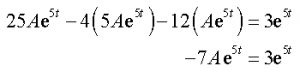
Now, all that we need to do is do a couple of derivatives, plug this into the differential equation and see if we can determine what A needs to be.

Plugging into the differential equation gives

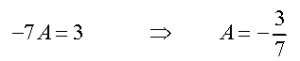
So, in order for our guess to be a solution we will need to choose A so that the coefficients of the exponentials on either side of the equal sign are the same. In other words we need to choose A so that,

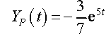
Okay, we found a value for the coefficient. This means that we guessed correctly. A particular solution to the differential equation is then,

Before continuing any further we should again take note of that we began off the arrangement above by discovering the corresponding arrangement. This is not actually part the technique for Undetermined Coefficients on the other hand, as we’ll in the long run see, having this under control before we make our supposition for the specific arrangement can spare us a great deal of work and/or migraine. Discovering the corresponding arrangement first is basically a decent propensity to have.

We know that the general solution will be of the form,

In this way, we require the general answer for the nonhomogeneous differential comparison. Taking the integral arrangement and the specific arrangement that we found in the past case we get the accompanying for a general arrangement and its derivative.

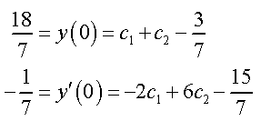
Now, apply the initial conditions to these.

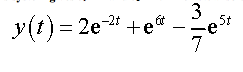
Solving this system gives c₁ = 2 and c₂ = 1. The actual solution is then.

here are some links from Khan Academy to help clarify the theory:

6 Comments

Posted in Uncategorized

Tagged differential equations, khan academy, Method of Undetermined Coefficients, Nonhomogeneous

Category Archives: Uncategorized

Taylor Series

Laplace Transform: Solution of the Initial Value Problems (Inverse Transform)

Improvements on the Euler Method (backwards Euler and Runge-Kutta)

Series Solutions around an ordinary point…. Taylor Series : Sec 5.2

Laplace Definition “Study Guide”

Importance of the “s” value: “s>0” and “s>a”

Fitting the equation into the Laplace transform table:

Laplace transform in 5 steps:

1. Start with a differential equation.

2. Take Laplace transformation of both sides.

3. Solve the resulting equation.

4. Simplify the solution.

5. Take the inverse Laplace.

Exam 3 Review – CORRECTIONS

Euler’s Method

Repeated Roots Second Order Linear Homogeneous Equation

Nonhomogeneous Method of Undetermined Coefficients

Related sites:

Handy Web Resources

Math StackExchange

Recent Posts

Recent Comments

Categories

Archives

Meta

The OpenLab at City Tech:A place to learn, work, and share

Support

Accessibility

Copyright

Creative Commons

The OpenLab at City Tech:A place to learn, work, and share

Support

Accessibility

Copyright

Creative Commons

Category Archives: Uncategorized

Importance of the “s” value: “s>0” and “s>a”

Fitting the equation into the Laplace transform table:

Laplace transform in 5 steps:

1. Start with a differential equation.

2. Take Laplace transformation of both sides.

3. Solve the resulting equation.

4. Simplify the solution.

5. Take the inverse Laplace.

Related sites:

Handy Web Resources

Recent Posts

Recent Comments

Categories

Archives

Meta

Tags

The OpenLab at City Tech:A place to learn, work, and share

Support

Accessibility

Copyright