Tag Archives: review

Definition of Laplace Transform

Posted on May 13, 2015 by Christian Pinto | 7 comments

Laplace transform is a method used to go from one domain to another domain. In this case we go from the time domain (t) to the frequency domain (s).

As for most conversions, if there is one way to go from one unit to another, there should be a way to go backwards. It applies in this case also, although it isn’t necessarily a unit. In this case it’s simply called “Inverse Laplace Transform”. In this case we go from the Frequency domain (s), back to the time domain (t).

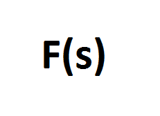
The notation for the Laplace transform is:

$\mathcal{L}\{f(t)\}$

The “L” is used to denote Laplace transform. What is inside the curly braces is the function you want to transform from the time domain to the frequency domain.

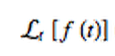
You may sometimes also see this notation which means the same as the one before:

As for the Laplace transform, it is denoted:

This will give you F(s).

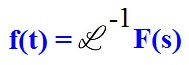
In order to get to the original time domain, you need to take the inverse Laplace transform of F(s) which is:

Now that we got the notation down for the Laplace transform we can go into more depth.

The general formula for the Laplace transform where ‘t’ is greater than or equal to zero:

$F(s) =\int_0^{\infty} e^{-st} f(t)\, dt.$ We evaluate at t is greater than or equal to zero because we want to satisfy two conditions:

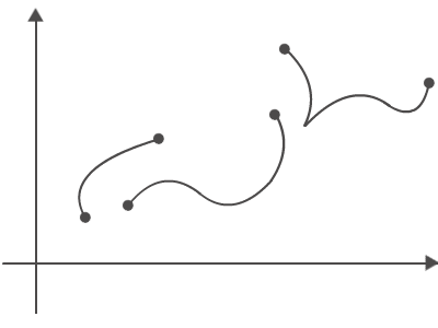
1. The function f(t) has to be piecewise continuous from the interval [0,A]. Simply means a function that is broken apart into different pieces but still continues on. For example:

2. The same function f(t) must be of exponential order. This means that the function f(t) must be smaller than or equal to ke^(at) when t is grater than or equal to M. In this case the variables K, M, and a are just constants and K, M are positive.

As for the inverse Laplace transform, there isn’t any set equation or method of doing it. The way the inverse Laplace transform is denoted, is by the following:

It simply mean to get the function f(t) you would need to take the inverse Laplace transform of F(s).

The main reason we use Laplace transform is because it makes certain (not all) differential equations easier.

A small introduction on the steps to take when solving a Laplace transform problem. There are five steps that we can use to solve a differential equation using Laplace transform:

1. Have a differential equation to solve

2. Take the Laplace transform of both sides in the equation. This will give you a simple algebraic equation to solve.

3. Solve the algebraic equation

4. Simplify the algebraic so you have what you are solving for on the left side and what it is equal to on the right side. If you can simplify the right side it will make it easier. Once simplified use partial fractions to solve for the unknowns.

5. Take the inverse Laplace transform and you will have your solution for the differential equation.

7 Comments

Posted in Resources, Study Guide

Tagged differential equations, Laplace, review

Final Exam Review is posted

Posted on May 12, 2015 by Jonas Reitz | Leave a comment

Hi everyone,

The review sheet for the final exam is posted on the Handouts page.

Best,
Prof. Reitz

Study Guide: Second Order Linear Homogeneous Equations with Constant Coefficients

Posted on April 29, 2015 by MattiiE | Leave a comment

What is Second Order Linear Homogeneous Equations with Constants Coefficients?

A second order homogeneous equation with constant coefficients is written as:

$Ay''+By'+Cy=0$ where A, B, C are constant and $A\neq0$

In order to solve these equation, we would convert the differential equation into a characteristic equation which is something like this:

$Ar^2+Br+C=0$

Then we use the quadratic equation to find the roots for the equation:

$r_{1,2}= \frac{-B\pm\sqrt{B^2-4AC}}{2A}$

There are three cases will be distinguish by using the discriminant ( $D=B^2-4AC$ ), after getting the discriminant then we apply the roots in to their own general solution, such that:

$D>0$ (there will be two distinct real roots, $r_1$ and $r_2$ )
$y(t)= K_1e^{r_1t} + K_2e^{r_2t}$
$D=0$ (there will be one repeated root, $r_1=r_2$ )
$y(t)= K_1e^{r_1t} + K_2te^{r_2t}$
$D<0$ (there will be two complex roots, $r_{1,2}=\alpha \pm i\beta$ )
$y(t)= K_1e^{\alpha t}\cos(\beta t) + K_2e^{\alpha t}\sin(\beta t)$

Sample Problem:
Find the solution for the following equation:

$y''-6y'+9y=0, y(o)=-5, y'(0)=-4$

Step 1: Converting the differential equation into characteristic equation and distinguish A, B and C.

$r^2-6r+9y=0$
where $A=1,B=-6,C=9$

Step 2: Distinguish which case will the equation be with the discriminant.

$D=(-6)^2-4(1)(9)$
$D=36-36$
$D=0$

In this case, we will be looking into an equation with a repeated root. So our general solution will look something like this:

$y(t)= K_1e^{r_1t} + K_2te^{r_2t}$

Step 3: Using the quadratic equation to solve for $r_{1,2}$ or you can solve it by factoring if it’s possible(in this case factoring is possible).
By factoring:

$r^2-6r+9y=0$
$(r-3)(r-3)=0$
$r_1=r_2=3$

By quadratic equation:

$r_{1,2}= \frac{-(-6)\pm\sqrt{(-6)^2-4(1)(9)}}{2(1)}$

$r_{1,2}= \frac{6\pm\sqrt{36-36}}{2}$

$r_{1,2}= \frac{6}{2}$

$r_{1,2}= 3$

Step 4:After solving for the roots, now we apply the roots into the general solution.

$y(t) = K_1e^{3t} + K_2te^{3t}$

Step 5:Then we solve for the constant( $K_1, K_2$ )using the initial values that are given to us.

$y(o)=-5, y'(0)=-4$

$y(t) = K_1e^{3t} + K_2te^{3t}$

Also we need to find the first derivatives of the equation.

$y'(t) = 3K_1e^{3t} + K_2e^{3t} + 3K_2te^{3t}$

By using the initial values we will then able to solve for $K_1,K_2$ .

$y(0) = K_1e^{3(0)} + K_2(0)e^{3(0)}=-5$
$K_1=-5$

$y'(0) = 3(-5)e^{3(0)} + K_2e^{3(0)} + 3K_2(0)e^{3(0)}=-4$
$K_2=11$

Lastly we apply the constant back into the equation and we will have the final solution for this problem.

$y(t) = -5e^{3t} + 11te^{3t}$

Videos for reference:
Here are some videos that I think will be useful to look at.
Introduction of Second Order Linear Homogeneous Equations with Constant Coefficients:

Second Order Linear Homogeneous Equations with Constant Coefficients with two distinct real roots:

Second Order Linear Homogeneous Equations with Constant Coefficients with repeated roots:

Second Order Linear Homogeneous Equations with Constant Coefficients with two complex roots:

*I don’t own these videos, all credits goes to the you-tuber Houston Math Prep.*

Exam 1 Review is posted

Posted on February 21, 2015 by Jonas Reitz | 2 comments

Hi everyone,

Exam #1 will take place on Thursday, March 5th, during class. The review sheet for Exam #1 has been posted on the “Handouts” page. Let me know if you have any questions.

Regards,
Prof. Reitz

2 Comments

Posted in Resources

Tagged answer key, exam, exam 1 review, review

Calculus Review – some helpful hints for WeBWorK #1

Posted on February 1, 2015 by Jonas Reitz | 2 comments

EDIT 2/2/15: Added an example for finding the tangent line to a function.

Having trouble with the WeBWorK? First, don’t panic – it’s a lot to remember!! But do be prepared to put in some time re-learning stuff from Calculus I and II. I’ve picked out a few video resources for you that hit some of the most important techniques (I tried to find videos that were focussed on examples, rather than theory, since this is meant to be review).

Comments are welcome (just click the “leave a comment” button above).

Like a video? Leave comment and let me know.
Dislike a video (it wasn’t helpful/ it was confusing)? Let me know.
Need help with another topic (like the product rule, or equations of tangent lines, or something else)? Let me know.
Have a video or other resource to suggest? Let me know!

Derivatives: Equation of the tangent line to a curve (similar to Problem 2): This gives an example of finding the equation of a tangent line, starting with just the function and the x-value. (NOTE: In the video, the function is an exponential function, so the numbers running around the answer all tend to have e in them – this will not be the case in the WeBWorK problem, where you will find more familiar numbers in your answer).

Derivatives: The Chain Rule (similar to Problem 4): This video is short and sweet, a single example using the chain rule with a logarithmic function.

Integrals: U-Substitution (similar to Problems 5 & 6):

This video has three examples – the first two are most similar to what you will see in WeBWorK (the last one is a little trickier – but could be useful in the future):

Integration by Parts (similar to Problems 7 & 8)

This video also has a few examples – the first two will be most useful for the WeBWorK:

2 Comments

Posted in Resources

Tagged calculus, chain rule, differentiation, integration, integration by parts, review, substitution, videos

Tag Archives: review

Definition of Laplace Transform

Final Exam Review is posted

Study Guide: Second Order Linear Homogeneous Equations with Constant Coefficients

Exam 1 Review is posted

Calculus Review – some helpful hints for WeBWorK #1

Related sites:

Handy Web Resources

Math StackExchange

Recent Posts

Recent Comments

Categories

Archives

Meta

The OpenLab at City Tech:A place to learn, work, and share

Support

Accessibility

Copyright

Creative Commons

The OpenLab at City Tech:A place to learn, work, and share

Support

Accessibility

Copyright

Creative Commons

Tag Archives: review

Related sites:

Handy Web Resources

Recent Posts

Recent Comments

Categories

Archives

Meta

Tags

The OpenLab at City Tech:A place to learn, work, and share

Support

Accessibility

Copyright