Tag Archives: Laplace

Laplace Transform: Solution of the Initial Value Problems (Inverse Transform)

The Laplace transform is an important technique in differential equations, and it is also widely used a lot in electrical engineering to solving linear differential equation The Laplace transform takes a function whose domain is in time and transforms it into a function of complex frequency.

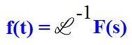
The inverse Laplace transform does exactly the opposite, it takes a function whose domain is in complex frequency and gives a function defined in the time domain.

The steps to using the Laplace and inverse Laplace transform with an initial value are as follows:

1) We need to know the transformations we have to apply, which are:

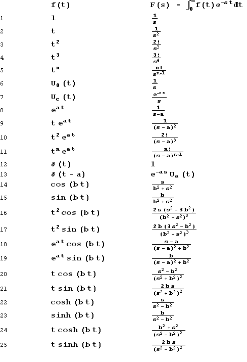
L{y’}=sY(s)-y(0)                     L{y”}=s^2 Y(s)-sy(0)-y'(0)

2) Once we apply the proper Laplace transform to our function we then apply the initial condition

3)Then since we can’t find y(t) directly, we solve for Y(s), which is the Laplace transform of y(t)

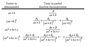
4) Once we find Y(s), we may need to break up the equation into partial fraction form depending on the denominator. there must only be a single term in the denominator and no “s” in the numerator. (look at “Factor in Denominator” chart image attached)

5) We take the inverse Laplace transform to get y(t)


So now to apply those steps,

Let’s take for example, 2y’-y = 1 ; y(0) = 0

1) Apply the transforms.                                 2(sY(s)-y(0))-Y(s)= 1/s

2) Apply the initial conditions given.               2(sY(s)-0)-Y(s)= 1/s

3) Solve for Y(s).                                            Y(s)(2s-1) = 1/s                     Y(s)=1/s(2s-1)

4) Apply the inverse transform.                   L^(-1){1/s(2s-1)} = L^(-1){1/(2s-1)-(1/s)}   =   e^(1/2t)-1


For another example, let’s take something that requires us to use partial fractions to get the right denominator.

F(s) = [19/(s+2)]-[1/(3s-5)]+[7/(s^5)]


So to get started on this one, we look at the Laplace transform table and see which fraction refers to the transformation. The first fraction looks like 1/(s-a) = e^(at). Although the “a” in this case would be a -2. For the second fraction, we got the same case except that the s is 3s, so all we have to do is factor out the 3, and apply the Laplace transform. And for the third fraction we see that it looks like, (n!)/s^(n+1) = t^n ; and since the exponent in the denominator is 5, the value for n = 4. But now we still have a 7 in the numerator whereas we need a 4! or 24. So to fix this all we have to do is multiply the top numerator by a constant to achieve the desired numerator, but we have to remember to divide by the same constant after taking the Laplace transform.


So it would be:

F(s) = [19/(s-(-2))]-[1/3(s-(5/3))]+[7(4!/4!)/(s^(4+1))]

So, now we have to take the inverse Laplace transform.

f(s) = 19e^(-2t) – (1/3)e^(5t/3) + 7/24(t^4)

I hope that the link to the video and images are helpful.

https://www.khanacademy.org/math/differential-equations/laplace-transform/laplace-transform-to-solve-differential-equation/v/laplace-transform-to-solve-an-equation

Untitled 2


Definition of Laplace Transform

Laplace transform is a method used to go from one domain to another domain. In this case we go from the time domain (t) to the frequency domain  (s).

As for most conversions, if there is one way to go from one unit to another, there should be a way to go backwards. It applies in this case also, although it isn’t necessarily a unit. In this case it’s simply called “Inverse Laplace Transform”. In this case we go from the Frequency domain (s), back to the time domain (t).

The notation for the Laplace transform is:

\mathcal{L}\{f(t)\}

The “L” is used to denote Laplace transform. What is inside the curly braces is the function you want to transform from the time domain to the frequency domain.

You may sometimes also see this notation which means the same as the one before:

fs

As for the Laplace transform, it is denoted:

Capture

This will give you F(s).

In order to get to the original time domain, you need to take the inverse Laplace transform of  F(s) which is:

eq0001MP

Now that we got the notation down for the Laplace transform we can go into more depth.

The general formula for the Laplace transform where ‘t’ is greater than or equal to zero:

F(s) =\int_0^{\infty} e^{-st} f(t)\, dt. We evaluate at t is greater than or equal to zero because we want to satisfy two conditions:

1. The function f(t) has to be piecewise continuous from the interval [0,A]. Simply means a function that is broken apart into different pieces but still continues on. For example:

piecewise-continuous


2. The same function f(t) must be of exponential order. This means that the function f(t) must be smaller than or equal to ke^(at) when t is grater than or equal to M. In this case the variables K, M, and a are just constants and K, M are positive.

As for the inverse Laplace transform, there isn’t any set equation or method of doing it. The way the inverse Laplace transform is denoted, is by the following:

laplace-transformation

It simply mean to get the function f(t) you would need to take the inverse Laplace transform of F(s).

The main reason we use Laplace transform is because it makes certain (not all) differential equations easier.

A small introduction on the steps to take when solving a Laplace transform problem. There are five steps that we can use to solve a differential equation using Laplace transform:

1. Have a differential equation to solve

2. Take the Laplace transform of both sides in the equation. This will give you a simple algebraic equation to solve.

3. Solve the algebraic equation

4. Simplify the algebraic so you have what you are solving for on the left side and what it is equal to on the right side. If you can simplify the right side it will make it easier. Once simplified use partial fractions to solve for the unknowns.

5. Take the inverse Laplace transform and you will have your solution for the differential equation.