Tag Archives: khan academy

Repeated Roots Second Order Linear Homogeneous Equation

Overview

Second order linear equations become homogeneous when the linear function of y and y’ (which can be written in the form y” + p(t)y’ + q(t)y = g(t)) is equal to zero. In other words when g(t)=0.

This guide will be discussing how to solve homogeneous linear second order differential equation with constant coefficient, which is written in the following form:

y”+by’+cy = 0

The first step is to use the equation above to turn the differential equation into a characteristic    equation. The characteristic equation is written in the following form:

r2 +br+c = 0

Second to find the roots, or r1 and r2 you can either factor or use the quadratic formula:

 r2 = ± -b √b²-4ac

 2a

It is important to remember when to the particular equation above. There will problems where the variable a is not needed in the quadratic formula because there will be no a in the differential equation. In the cases where there is no a variable limit the a variable from the quadratic equation. The quadratic equation will the look like the following:

r2 = ± -b √b²-4c

2

Once you get repeated roots , or r1 and r2 from the characteristic equation then     y = ert is considered a solution of the differential equation.

The next step would be to plug r1 and r2 into the general equation:

y = C1 er1t +C2 er2t

Another important thing to realize and remember is that when solving a homogeneous equation for a repeated root the solution will end up cancelling out. In order to avoid this a “t” needs to be place in the general solution. The general solution for the repeated root will then be in the following form:

y = C1 er1t +C2t er2t

Sample Problem

Problem 1:

y”+12y’+36 = 0

Step 1: Turn the differential equation into a characteristic equation

r2 + br + c = 0

r2 + 12r + 36 = 0

Step 2: Factor the characteristic equation

r2 + 12r + 36 = 0

(r + 6) (r + 6) = 0

r1 = -6 r2 = -6

Step 3: Use y = ert as a solution for r1 and r2

y = ert

y = e-6t

Step 4: Plug r1 and r2 into the general solution for the repeated roots

y = C1 er1t +C2t er2t

y = ert

y = e-4t

Step 4: Plug r1 and r2 into the general solution for the repeated roots

y = C1 er1t +C2t er2t

y = C1 e-4t +C2t e-4t

y = C1 e-6t +C2t e-6t


Problem 2:

y”+8y’+16 = 0 , y(0) = 2   y’(0)= 6

Step 1: Turn the differential equation into a characteristic equation

r2 + br + c = 0

r2 + 8r + 16 = 0

Step 2: Factor the characteristic equation

r2 + 8r + 16 = 0

(r + 4) (r + 4) = 0

r1 = -4 r2 = -4

Step 3: Use y = ert as a solution for r1 and r2

y = ert

y = e-4t

Step 4: Plug r1 and r2 into the general solution for the repeated roots

y = C1 er1t +C2t er2t

y = C1 e-4t +C2t e-4t

The following three videos are form Khan Academy. I find these videos ever useful . I would recommend you watch them if you are still confused  about Repeated Roots of Second order linear homogeneous equation.


Nonhomogeneous Method of Undetermined Coefficients

Nonhomogeneous Method of Undetermined Coefficients

 In this area we will investigate the first technique that can be utilized to locate a specific answer for a nonhomogeneous differential mathematical statement.

Screen Shot 2015-04-30 at 10.15.48 PM  One of the primary points of interest of this strategy is that it diminishes the issue down to a polynomial math issue. The variable based math can get untidy every so often, however for the majority of the issues it won’t be appallingly troublesome. Another decent thing about this system is that the corresponding arrangement won’t be unequivocally needed, albeit as we will see information of the reciprocal arrangement will be required now and again thus we’ll by and large find that also. There are two inconveniences to this system. To begin with, it will work for a genuinely little class of g(t)’s. The class of g(t) for which the technique works, does incorporate a percentage of the more basic capacities, nonetheless, there are numerous capacities out there for which undetermined coefficients just won’t work. Second, it is by and large helpful for consistent coefficient differential mathematical statements.

 The technique is truly straightforward. All that we have to do is take a gander at g(t) and make a speculation as to the type of YP(t) leaving the coefficient(s) undetermined (and thus the name of the system). Plug the conjecture into the differential mathematical statement and check whether we can focus estimations of the coefficients. In the event that we can focus values for the coefficients then we speculated effectively, on the off chance that we can’t discover qualities for the coefficients then we speculated inaccurately.

 let’s jump into example:


Screen Shot 2015-04-30 at 10.15.53 PM                                     

The point here is to find a particular solution, however the first thing that we’re going to do is find the complementary solution to this differential equation.  Recall that the complementary solution comes from solving,                                             

Screen Shot 2015-04-30 at 10.16.03 PMThe characteristic equation for this differential equation and its roots are.

                        Screen Shot 2015-04-30 at 10.16.11 PM

 The complementary solution is then,

                                          Screen Shot 2015-04-30 at 10.16.18 PM

 The technique is truly straightforward. All that we have to do is take a gander at g(t) and make a speculation as to the type of YP(t) leaving the coefficient(s) undetermined (and thus the name of the system). Plug the conjecture into the differential mathematical statement and check whether we can focus estimations of the coefficients. In the event that we can focus values for the coefficients then we speculated effectively, on the off chance that we can’t discover qualities for the coefficients then we speculated inaccurately.

 Presently, how about we continue with discovering a specific arrangement. As said proceeding the begin of this case we have to make a supposition as to the type of a specific answer for this differential mathematical statement. Since g(t) is an exponential and we realize that exponentials never simply show up or vanish in the separation process it appears that a possible type of the specific arrangement would be.

                                                Screen Shot 2015-04-30 at 10.16.26 PM

 Now, all that we need to do is do a couple of derivatives, plug this into the differential equation and see if we can determine what A needs to be. 

 Plugging into the differential equation gives

                                            Screen Shot 2015-04-30 at 10.16.42 PM

 So, in order for our guess to be a solution we will need to choose A so that the coefficients of the exponentials on either side of the equal sign are the same.  In other words we need to choose A so that,

                                                Screen Shot 2015-04-30 at 10.16.49 PM

 Okay, we found a value for the coefficient.  This means that we guessed correctly.  A particular solution to the differential equation is then,

Screen Shot 2015-04-30 at 10.16.57 PM

Before continuing any further we should again take note of that we began off the arrangement above by discovering the corresponding arrangement. This is not actually part the technique for Undetermined Coefficients on the other hand, as we’ll in the long run see, having this under control before we make our supposition for the specific arrangement can spare us a great deal of work and/or migraine. Discovering the corresponding arrangement first is basically a decent propensity to have.


Screen Shot 2015-04-30 at 10.17.05 PM 

We know that the general solution will be of the form,

                            Screen Shot 2015-04-30 at 10.17.13 PM                             

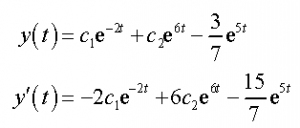
 In this way, we require the general answer for the nonhomogeneous differential comparison. Taking the integral arrangement and the specific arrangement that we found in the past case we get the accompanying for a general arrangement and its derivative.

  Screen Shot 2015-04-30 at 10.17.21 PM

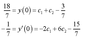
Now, apply the initial conditions to these.

   Screen Shot 2015-04-30 at 10.17.28 PM

Solving this system gives c1 = 2 and c2 = 1.  The actual solution is then.

                     Screen Shot 2015-04-30 at 10.17.34 PM

here are some links from Khan Academy to help clarify the theory:


Second order ordinary homogeneous differential equations with constant coefficients

Here are some video resources showing complete examples (from Khan Academy).  I hope they help!

-Prof. Reitz

Example 1 — in which the characteristic equation has two distinct real roots.


Example 2 — in which the characteristic equation has one repeated (real) root.


Example 3 — in which the characteristic equation has complex roots.