Category Archives: Resources

Getting Started, How-Tos, and so on

Final Grades are posted

Posted on May 26, 2015 by Jonas Reitz | Leave a comment

Hi everyone,

Final grades for the course have been submitted to CUNYFirst, and a detailed breakdown of your grade (including your final exam score, your “Study Guide” project score, and so on) can be found on the GRADES page.

I wish you the very best in your future endeavors – it was a pleasure working with you this semester.

Best regards,
Prof. Reitz

Leave a comment

Posted in Resources

Tagged farewell, final, grades

Final Exam Review CORRECTION

Posted on May 17, 2015 by Jonas Reitz | 2 comments

Hi everyone,

I’ve updated the answer to problem #14 – the correct answer is:

$Q(t)=1.31317e^{-4t}\sin(7.31057t)+2.4e^{-4t}\cos(7.31057t)$

$I(t)=-22.798e^{-4t}\sin(7.31057t)$

Best,
Prof. Reitz

2 Comments

Posted in Resources

Tagged correction, final exam review

Exam 3 Grades are posted, and SPECIAL OFFER

Posted on May 16, 2015 by Jonas Reitz | Leave a comment

Hi everyone,

The grades for Exam 3 are posted on the Grades page (email me if you have forgotten the password).

This exam covered a great deal of material and, while overall grades were comparable to the first exam, I’m sure not everyone did as well as they would have liked. You may improve your score on the exam by completing the Special Offer below.

Let me know if you have any questions, and best of luck with your studying!
Prof. Reitz

Exam 3 Special Offer – earn bonus points. You can improve your grade on the exam, by doing the following:

Choose ONLY ONE problem in which you did NOT earn full points. You are working to earn back (some of ) the points you missed on this problem.
Do the problem over, neatly and completely, start to finish, on a separate sheet of paper.
1. Don’t forget your name, the date, and the problem number.
On the same sheet, write a short statement (one or two complete sentences) explaining your mistake(s) – the purpose is to let me know that you understand what you did wrong.
Hand in your original exam and your corrected problem and explanation, stapled together, in class on Thursday (the day of the final exam).
Bonus points will be added to your Exam 3 score based on the number of points you missed on the chosen problem, the accuracy of your corrections and explanation, and your overall grade on the exam. Bonus points are limited as follows:
1. If you received less than 60% on the exam, you can earn a maximum of 20 bonus points.
2. If you received between 60% – 69% on the exam, you can earn a maximum of 15 bonus points.
3. If you received between 70% – 79% on the exam, you can earn a maximum of 10 bonus points.
4. If you received between 80% – 89% on the exam, you can earn a maximum of 5 bonus points.
5. If you received between 90% or more on the exam, you can earn a maximum of 2 bonus points.

Leave a comment

Posted in Assignments, Resources

Tagged exam 3, grades, special offer

Definition of Laplace Transform

Posted on May 13, 2015 by Christian Pinto | 7 comments

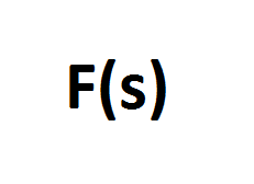
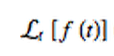
Laplace transform is a method used to go from one domain to another domain. In this case we go from the time domain (t) to the frequency domain (s).

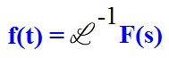
As for most conversions, if there is one way to go from one unit to another, there should be a way to go backwards. It applies in this case also, although it isn’t necessarily a unit. In this case it’s simply called “Inverse Laplace Transform”. In this case we go from the Frequency domain (s), back to the time domain (t).

The notation for the Laplace transform is:

$\mathcal{L}\{f(t)\}$

The “L” is used to denote Laplace transform. What is inside the curly braces is the function you want to transform from the time domain to the frequency domain.

You may sometimes also see this notation which means the same as the one before:

As for the Laplace transform, it is denoted:

This will give you F(s).

In order to get to the original time domain, you need to take the inverse Laplace transform of F(s) which is:

Now that we got the notation down for the Laplace transform we can go into more depth.

The general formula for the Laplace transform where ‘t’ is greater than or equal to zero:

$F(s) =\int_0^{\infty} e^{-st} f(t)\, dt.$ We evaluate at t is greater than or equal to zero because we want to satisfy two conditions:

1. The function f(t) has to be piecewise continuous from the interval [0,A]. Simply means a function that is broken apart into different pieces but still continues on. For example:

2. The same function f(t) must be of exponential order. This means that the function f(t) must be smaller than or equal to ke^(at) when t is grater than or equal to M. In this case the variables K, M, and a are just constants and K, M are positive.

As for the inverse Laplace transform, there isn’t any set equation or method of doing it. The way the inverse Laplace transform is denoted, is by the following:

It simply mean to get the function f(t) you would need to take the inverse Laplace transform of F(s).

The main reason we use Laplace transform is because it makes certain (not all) differential equations easier.

A small introduction on the steps to take when solving a Laplace transform problem. There are five steps that we can use to solve a differential equation using Laplace transform:

1. Have a differential equation to solve

2. Take the Laplace transform of both sides in the equation. This will give you a simple algebraic equation to solve.

3. Solve the algebraic equation

4. Simplify the algebraic so you have what you are solving for on the left side and what it is equal to on the right side. If you can simplify the right side it will make it easier. Once simplified use partial fractions to solve for the unknowns.

5. Take the inverse Laplace transform and you will have your solution for the differential equation.

7 Comments

Posted in Resources, Study Guide

Tagged differential equations, Laplace, review

Final Exam Review is posted

Posted on May 12, 2015 by Jonas Reitz | Leave a comment

Hi everyone,

The review sheet for the final exam is posted on the Handouts page.

Best,
Prof. Reitz

Leave a comment

Posted in Resources

Tagged final exam, review

Exam 3 Review – Problem 2 STEP BY STEP (Taylor Series)

Posted on May 9, 2015 by Jonas Reitz | 1 comment

Hi everyone – here is a step-by-step solution to Problem 2 from the Exam 3 Review. If you have any questions (or notice an error), please leave a comment in reply to this post.

2. Given the differential equation $y''-xy'-y=0$ ,

a. Suppose that $y(x)$ has a Taylor series about $x=0$ , $y(x)=\sum\limits_{n=0}^{\infty} \frac{f^{(n)}(0)}{n!} x^n=a_0+a_1 x + a_2 x^2 + a_3 x^3 + a_4 x^4 +\ldots$ Substitute into the differential equation and simplify by grouping together terms with similar powers of $x$ .

We start with the assumption that $y(x)= a_0+a_1 x + a_2 x^2 + a_3 x^3 + a_4 x^4 +\ldots$ . Find the first and second derivatives:

$y'(x)= a_1+2a_2x+3a_3x^2+4a_4x^3+\ldots$
$y''(x)= 2a_2+6a_3x+12a_4x^2+\ldots$

Now substitute $y, y'$ and $y''$ into the differential equation $y''-xy'-y=0$ :

$(2a_2+6a_3x+12a_4x^2+\ldots)-x(a_1+2a_2x+3a_3x^2+4a_4x^3+\ldots)-(a_0+a_1 x + a_2 x^2 + a_3 x^3 + a_4 x^4 +\ldots)=0$

Get rid of parentheses (don’t forget to distribute the $-x$ and the $-$ in front of the second and third sets of parentheses):

$2a_2+6a_3x+12a_4x^2+\ldots-a_1x-2a_2x^2-3a_3x^3-4a_4x^4-\ldots-a_0-a_1 x-a_2 x^2-a_3 x^3-a_4 x^4-\ldots=0$

Now group together by powers of $x$ :

$(2a_2-a_0)+(6a_3x-a_1x-a_1x)+(12a_4x^2-2a_2x^2-a_2x^2)+\ldots=0$

(Remember, there is more stuff hidden in the “ $\ldots$ ” – if we wanted to, we could write down more terms of $y, y'$ and $y''$ and therefore get more terms here as well).

Finally, simplify each set of parentheses and factor out $x$ :

$(2a_2-a_0)+(6a_3-2a_1)x+(12a_4-3a_2)x^2+\ldots=0$

Finally, we compare each term on the left with the corresponding term on the right – since the right side is zero, each of the expressions in the parentheses (which give the coefficients of the powers of $x$ ) must also be equal to zero:

$2a_2-a_0=0$
$6a_3-2a_1=0$
$12a_4-3a_2=0$
$\ldots$

b. Given the initial conditions $y(0)=16, y'(0)=15$ , find the first five terms of the Taylor series solution $y(x)$ .

We need to find the coefficients $a_0, a_1, a_2, a_3, a_4, \ldots$ . The first two coefficients are given by $a_0 = y(0)=16$ and $a_1 = y(1)=15$ , so we have:

$a_0 = 16$
$a_1 = 15$
$a_2 = ?$
$a_3 = ?$
$a_4 = ?$
$\ldots$

To find the remaining coefficients, we use the equations we found at the end of part a) above, and solve each one for the unknown coefficient:

$2a_2-a_0=0$ becomes $a_2 = \frac{a_0}{2}$
$6a_3-2a_1=0$ becomes $a_3 = \frac{a_1}{3}$
$12a_4-3a_2=0$ becomes $a_4 = \frac{a_2}{4}$
$\ldots$

Substituting $a_0 = 16$ into the first equation gives $a_2 = 8$ .
Substituting $a_1 = 15$ into the second equation gives $a_3 = 5$ .
Substituting $a_2=8$ into the third equation gives $a_4 = 2$ .
$\ldots$

This gives us enough coefficients to determine the first five terms of the Taylor Series. Remembering that $y(x)= a_0+a_1 x + a_2 x^2 + a_3 x^3 + a_4 x^4 +\ldots$ , we substitute in the values of $a_0, a_1, a_2, a_3, a_4$ to obtain:

$y(x) \approx16+15x+8x^2+5x^3+2x^4$

NOTE: Since we have only given the first five terms of the Taylor series, the resulting expression is only an approximation of $y(x)$ — in order to make it exactly equal to $y(x)$ we would need to give all infinitely many terms. This is why we replace the equals sign with the ‘wavy equals’. (Note that I also dropped the $\ldots$ at the end).

c. Use the answer to part b to obtain an approximation of $y(2)$

Here, we just substitute $x=2$ into the expression we obtained above:

$y(2) \approx16+15\cdot 2+8\cdot 2^2+5\cdot 2^3+2\cdot 2^4=150$

1 Comment

Posted in Resources

Tagged exam 3 review, problem 2, step-by-step, Taylor Series

Partial Fractions: What if the top has a higher power than the bottom?

Posted on May 1, 2015 by Jonas Reitz | 2 comments

Partial fractions decomposition only works when the numerator has a smaller degree than the denominator. For example, here:

$\frac{s^2-s-9}{s-4}$

the numerator has degree 2 (because of the s-squared), and the denominator has degree 1, so partial fractions won’t work. What do we do? We need to divide the top by the bottom, using polynomial long division (this is another trick you may or may not remember from Algebra). When we are done, we get:

$\frac{s^2-s-9}{s-4} = s+3+\frac{3}{s-4}$

and we can proceed to take the Inverse Laplace Transform of the expression on the right.

To see how long division works for polynomials, check out these videos:

Basic examples:

Another example:

Best of luck – write back if you get stuck.
-Prof. Reitz

2 Comments

Posted in Resources

Tagged improper fractions, partial fractions, polynomial long division

Exam 3 Review is posted

Posted on May 1, 2015 by Jonas Reitz | Leave a comment

Hi everyone,

The review sheet for Exam #3 is posted on the Handouts page.

NOTE: You will be provided with a two-page formula sheet for use on the exam. This formula sheet appears on pages 2-3 of the Exam 3 Review. The final page of the Review contains the solutions.

Let me know if you have any questions.

Regards,
Prof. Reitz

Leave a comment

Posted in Resources

Tagged exam 3 review

Study Guide to Bernoulli Equations

Posted on April 30, 2015 by Compton Tudor | 1 comment

Overview

What are Bernoulli Equations?

Well to put it simply Bernoulli Equations are first order differential equations. What sets Bernoulli Equations apart from other first order differential equations is that they are nonlinear first order differential equation. When we was first introduced to first order differential equations we learned that the standard form was :

y’ +p(t)y = g(t) , y(to) = yo

What separates Bernoulli Equations from other first order equations is that in standard form, it is not equal to some function that is linear but one that has an exact solution. What this means is that their is some power that is raised to the right side of the equation which we shall call n and n cannot be equal to 0 or 1. this is what makes Bernoulli Equations nonlinear. Now we can change the form of a standard first order linear equation into a nonlinear first order equation:

y’ +p(t)y = q(t)y^(n) y(to)=yo

The above equation is now the standard form for a Bernoulli equation. What we can now understand from this equation is that p(t) and q(t) are functions that are continuous. Since n is a real number that has to be n> 0 and n>1 for this to be non linear.

Now the question is how do we solve Bernoulli Equations?

Sample Problem:

take an equation such as t^(2)y’ + 2ty – y^(3) = 0

and change it by adding y^(3) on both sides and we get:

t^(2)y’ + 2ty = y^(3)

Next we divide by t^(2) to on both sides of the equation so we can get it into standard form.

y’ + 2/yt = y^(3)/t^(2) <————-STANDARD FORM

Now we can go into the steps to solve this equation;

1. Divide by y^(n)

y’/y^(3) + 2/yt/y^(3) = (y^(3)/t^(2))/y^(3)

we get: (y’ + 2/yt)/y^(3) = 1/t^(2)

2. We substitute v = y^(1-n)

Since y^(3)

we get:v = y^(1-3) = y^(-2)

now we can rearrange the formula to so we can substitute v into it by moving the y^(2) to the numerator and we get:

y’/y^(3) + 2y^(-2)/t = 1/t^(2)

y’/y^(3) + 2v/t = 1/t^(2) <——————-Substitute v for y^(2)

Before we move to the solve Step we need to take the Derivative of the substitution v = y^(-2)

d/dy y^(-2)

dv/dt = -2y^(-3) dy/dt

(-1/2)v’ = -2y’/y^(3)(-1/2)

Now we can substitute for y’/y^(3) with the above equations and we get:

(-1/2)v’ + (2/t)v = 1/t^(2) <—————– First order linear equation

next we use the method of intergrating factor which states

mu = e^ intergral of (-4/t) which is equal to 1/t^(4)

we then multiply both sides b\by Mu and get the equation:

(dv(t)/dt)/t^(4) + d/dt(1/t^(4))v = (-2/t^(6))

Next we intergrate both sides and we come to the final answer of

y(t) = +- Sqrt(5t)/sqrt(ct^(5) + 2)

Videos:

I \\

1 Comment

Posted in Resources, Study Guide

Tagged advice for the future, divide by y^n, exact solutions, first order non linear, integrating factors, partial derivatives, standard form, substitute V=y^(1-n)

Help with Partial Fraction Decomposition

Posted on April 23, 2015 by Jonas Reitz | 43 comments

Hi everyone,

As we launch into our next topic, you will see that one of the (forgotten?) skills you will need is that of re-writing a complicated fraction as a sum of simpler fractions (“partial fraction decomposition”). For those that need some extra help/reminder of this process, here are a couple of videos:

Partial Fraction Decomposition – a basic example. This is a good basic example.

https://www.youtube.com/watch?v=HZTv4zCgEnA

Partial Fraction Decomposition – another example. This is a slightly longer example, and it includes a good explanation of how to set up your partial fractions for different kinds of factors in the denominator.

https://www.youtube.com/watch?v=pZ9FfGy3Cfw

43 Comments

Posted in Resources

Tagged examples, partial fraction decomposition, partial fractions, videos

Category Archives: Resources

Final Grades are posted

Final Exam Review CORRECTION

Exam 3 Grades are posted, and SPECIAL OFFER

Definition of Laplace Transform

Final Exam Review is posted

Exam 3 Review – Problem 2 STEP BY STEP (Taylor Series)

Partial Fractions: What if the top has a higher power than the bottom?

Exam 3 Review is posted

Study Guide to Bernoulli Equations

Help with Partial Fraction Decomposition

Related sites:

Handy Web Resources

Math StackExchange

Recent Posts

Recent Comments

Categories

Archives

Meta

The OpenLab at City Tech:A place to learn, work, and share

Support

Accessibility

Copyright

Creative Commons

The OpenLab at City Tech:A place to learn, work, and share

Support

Accessibility

Copyright

Creative Commons

Category Archives: Resources

Related sites:

Handy Web Resources

Recent Posts

Recent Comments

Categories

Archives

Meta

Tags

The OpenLab at City Tech:A place to learn, work, and share

Support

Accessibility

Copyright