Tag Archives: differential equations

Improved Euler’s Method

Posted on May 17, 2015 by BingJing Zheng | 11 comments

As we proceed through the course, we are usually given a first-order differential equation that could be solved. However, there are a lot of problems that cannot be solved. The first order equations could be divided into the linear equation, separable equation, nonlinear equation, exact equation, homogeneous equation, Bernoulli equation, and non-homogeneous equations. However, most of the separable and exact equation cannot always be presented the solution in an explicit form. It’s hard to find the value for a particular point in the function. There are some of the equations that do not fall into any of the categories above. So we introduce the method called Euler’s Method. We will be able to use it to approximate the solutions to a differential equation. In the Euler method, we will be given a differential equation which is the slope of a function, and define a step size for the integral ( the smaller steps sizes you have, the more accurate approximation values you will be get ). We generate a new point by starting at an initial point, we plug in this point into the given function, this will be the slope of the initial point. Then, then next new point will be the $y_0$ plus step size h time the previously calculated slope. the general formula is, $y_(n+1)=y_n+hf(t_n,y_n)$ However, the error for the Euler’s Method depends on the step size. the only way to decrease the error is to reduce the step size, but it will increase the amount of calculations. it only roughly decreases the error by half.

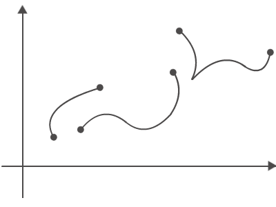
Now, we introduce an improved Euler’s Method. This method is quite similar to the Euler’s method. In the Euler’s Method we approximate the function by a rectangular shape (see graph below):

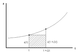
However, this approximate does not include the area that under the curve. To improve the approximation, we use the improved Euler’s method.The improved method, we use the average of the values at the initially given point and the new point. We define the integral with a trapezoid instead of a rectangle. The trapezoid has more area covered than the rectangle area. It will also provide a more accurate approximation.

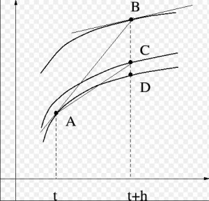
It is hard to predict the solution curve is concave up or concave down in reality. The ideal prediction line would exactly hit the curve at next predict point. The Euler’s Method generates the slope based on the initial point, and we don’t know if the next point will be on this slope line, unless we use a computer to plot the equation. Sometimes, we might overestimate the value or underestimate the value. The Improved Euler’s Method addressed these problems by finding the average of the slope based on the initial point and the slope of the new point, which will give an average point to estimate the value. It also decreases the errors that Euler’s Method would have.

The improved Euler’s Method simply divided into three steps as following:

Steps in Improved Euler’s Method:

Step 1 find the $k_1=f(t_n,y_n)$

Step 2 find the $k_2=f(t_n+h,y_n+hk_1)$

Step 3: find $y_(n+1)=f(t_n+h,y_n+h((k_1+k_2)/2))$

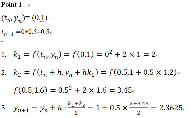
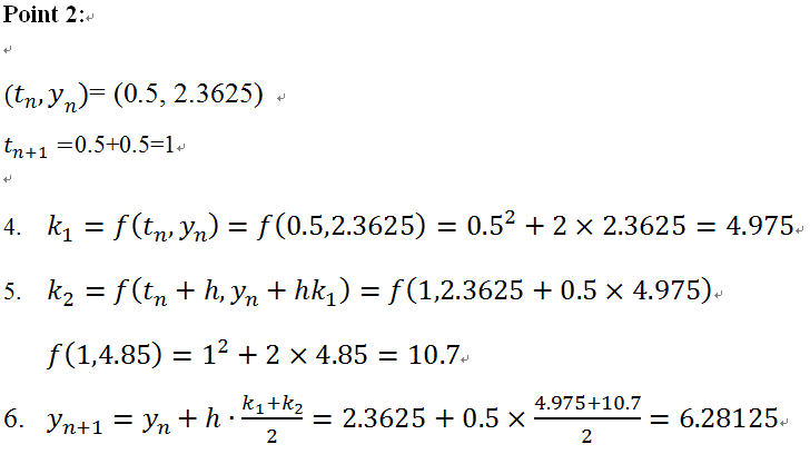
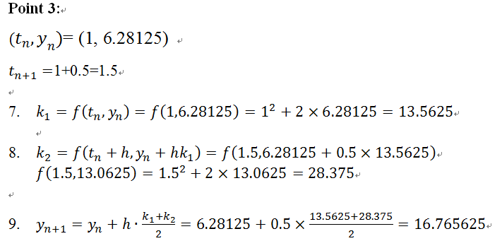
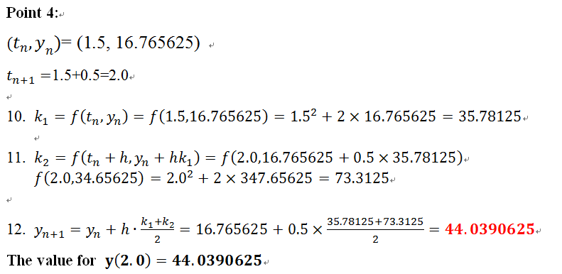
Given a first order linear equation y’=t^2+2y, y(0)=1, estimate y(2), step size is 0.5.

Summary

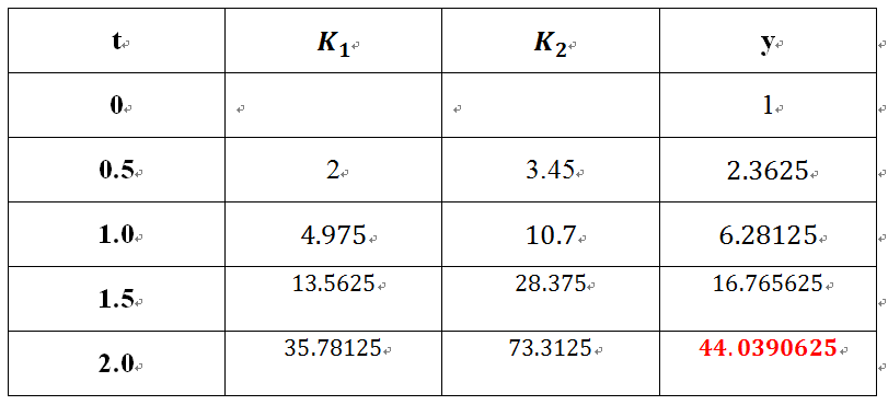
Note: it is very important to write the $(t_n,y_n)$ and $t_(n+1)$ at the beginning of each step because the calculations are all based on these values. This method involved with a lot of calculations, it is recommended after each point, write the values in a table. It will be easy for yourself to look up and check. For each point, the calculations approach to the next new point are the same, so if you set up the three steps, it will be very clear for you to continue to the next step.

I think this video is pretty helpful, and make a clear point on the improved Euler’s Method and a example include in the video. please check out this video.

11 Comments

Posted in Study Guide

Tagged Average slope, differential equations, Improved Euler's Method, Numerical Approximations: Euler’s Method Euler's Method

Definition of Laplace Transform

Posted on May 13, 2015 by Christian Pinto | 7 comments

Laplace transform is a method used to go from one domain to another domain. In this case we go from the time domain (t) to the frequency domain (s).

As for most conversions, if there is one way to go from one unit to another, there should be a way to go backwards. It applies in this case also, although it isn’t necessarily a unit. In this case it’s simply called “Inverse Laplace Transform”. In this case we go from the Frequency domain (s), back to the time domain (t).

The notation for the Laplace transform is:

$\mathcal{L}\{f(t)\}$

The “L” is used to denote Laplace transform. What is inside the curly braces is the function you want to transform from the time domain to the frequency domain.

You may sometimes also see this notation which means the same as the one before:

As for the Laplace transform, it is denoted:

This will give you F(s).

In order to get to the original time domain, you need to take the inverse Laplace transform of F(s) which is:

Now that we got the notation down for the Laplace transform we can go into more depth.

The general formula for the Laplace transform where ‘t’ is greater than or equal to zero:

$F(s) =\int_0^{\infty} e^{-st} f(t)\, dt.$ We evaluate at t is greater than or equal to zero because we want to satisfy two conditions:

1. The function f(t) has to be piecewise continuous from the interval [0,A]. Simply means a function that is broken apart into different pieces but still continues on. For example:

2. The same function f(t) must be of exponential order. This means that the function f(t) must be smaller than or equal to ke^(at) when t is grater than or equal to M. In this case the variables K, M, and a are just constants and K, M are positive.

As for the inverse Laplace transform, there isn’t any set equation or method of doing it. The way the inverse Laplace transform is denoted, is by the following:

It simply mean to get the function f(t) you would need to take the inverse Laplace transform of F(s).

The main reason we use Laplace transform is because it makes certain (not all) differential equations easier.

A small introduction on the steps to take when solving a Laplace transform problem. There are five steps that we can use to solve a differential equation using Laplace transform:

1. Have a differential equation to solve

2. Take the Laplace transform of both sides in the equation. This will give you a simple algebraic equation to solve.

3. Solve the algebraic equation

4. Simplify the algebraic so you have what you are solving for on the left side and what it is equal to on the right side. If you can simplify the right side it will make it easier. Once simplified use partial fractions to solve for the unknowns.

5. Take the inverse Laplace transform and you will have your solution for the differential equation.

7 Comments

Posted in Resources, Study Guide

Tagged differential equations, Laplace, review

Repeated Roots Second Order Linear Homogeneous Equation

Posted on May 1, 2015 by Carolina | 4 comments

Overview

Second order linear equations become homogeneous when the linear function of y and y’ (which can be written in the form y” + p(t)y’ + q(t)y = g(t)) is equal to zero. In other words when g(t)=0.

This guide will be discussing how to solve homogeneous linear second order differential equation with constant coefficient, which is written in the following form:

y”+by’+cy = 0

The first step is to use the equation above to turn the differential equation into a characteristic equation. The characteristic equation is written in the following form:

r² +br+c = 0

Second to find the roots, or r₁and r₂you can either factor or use the quadratic formula:

r² = ± -b √b²-4ac

It is important to remember when to the particular equation above. There will problems where the variable a is not needed in the quadratic formula because there will be no a in the differential equation. In the cases where there is no a variable limit the a variable from the quadratic equation. The quadratic equation will the look like the following:

r² = ± -b √b²-4c

Once you get repeated roots , or r₁ and r₂ from the characteristic equation then y = e^rt is considered a solution of the differential equation.

The next step would be to plug r₁ and r₂ into the general equation:

y = C₁ e^r1t +C₂ e^r2t

Another important thing to realize and remember is that when solving a homogeneous equation for a repeated root the solution will end up cancelling out. In order to avoid this a “t” needs to be place in the general solution. The general solution for the repeated root will then be in the following form:

y = C₁ e^r1t +C₂t e^r2t

Sample Problem

Problem 1:

y”+12y’+36 = 0

Step 1: Turn the differential equation into a characteristic equation

r² + br + c = 0

r² + 12r + 36 = 0

Step 2: Factor the characteristic equation

r² + 12r + 36 = 0

(r + 6) (r + 6) = 0

r₁ = -6 r₂ = -6

Step 3: Use y = e^rt as a solution for r₁ and r₂

y = e^rt

y = e^-6t

Step 4: Plug r₁ and r₂ into the general solution for the repeated roots

y = C₁ e^r1t +C₂t e^r2t

y = e^rt

y = e^-4t

Step 4: Plug r₁ and r₂ into the general solution for the repeated roots

y = C₁ e^r1t +C₂t e^r2t

y = C₁ e^-4t +C₂t e^-4t

y = C₁ e^-6t +C₂t e^-6t

Problem 2:

y”+8y’+16 = 0 , y(0) = 2 y’(0)= 6

Step 1: Turn the differential equation into a characteristic equation

r² + br + c = 0

r² + 8r + 16 = 0

Step 2: Factor the characteristic equation

r² + 8r + 16 = 0

(r + 4) (r + 4) = 0

r₁ = -4 r₂ = -4

Step 3: Use y = e^rt as a solution for r₁ and r₂

y = e^rt

y = e^-4t

Step 4: Plug r₁ and r₂ into the general solution for the repeated roots

y = C₁ e^r1t +C₂t e^r2t

y = C₁ e^-4t +C₂t e^-4t

The following three videos are form Khan Academy. I find these videos ever useful . I would recommend you watch them if you are still confused about Repeated Roots of Second order linear homogeneous equation.

4 Comments

Posted in Study Guide, Uncategorized

Tagged characteristic equation, differential equations, khan academy

Non-homogeneous Second Order Differential Equations Using Methods Of Undetermined Coefficients

Posted on May 1, 2015 by shawn chowdhury | 1 comment

Non-homogeneous differential equations are the same as homogeneous differential equations, However they can have terms involving only x, (and constants) on the right side. The interesting part of solving non homogeneous equations is having to guess your way through some parts of the solution process.
You also can write non-homogeneous differential equations in this format: y” + p(x)y’ + q(x)y = g(x).

The Reason I’ve chosen this problem is because it basically touches every aspect of a Non-homogeneous second order differential Equation using methods of undetermined coefficients.

y” + 6y’ + 9y = -578 sin 5t

The first step when dealing with undetermined or constant coefficients is getting the Characteristic equation. Which will later become the first half of our solution.

y” + 6y’ + 9y = 0
r^2 + 6r + 9 = 0
( r+3 ) ( r+3) = 0
R1 = -3 R2 = -3

When solving the characteristic equation sometimes we run into repeated roots. In this case we must use the following formula y = C1e^r1(t)+C2 (t)e^r2(t)

y (t) = C1e^-3t + C2te^-3t

After finding the characteristic equation our next step in this linear equation is to guess the y. In this case our y is going to include both sin and cosine. We make this guess because the cosine is going to come up eventually when finding the derivative and by adding it into the equation, it will allow us to cancel it out later on throughout the steps in the solution process. We also will need to find the y’ and y”.

y = C sin (5t) + D cos (5t)
y’ = 5 C cos (5t) – 5 D sin (5t)
y” = -25 C sin (5t) + 9 D cos (5t)

Now we plug it back into its original equation.

-25 C sin (5t) – 25 D cos (5t)
+30 C cos (5t) – 30 D sin (5t)
+9 C sin (5t) + 9 D sin (5t)
= -578 sin 5(t)

At this point we want to cancel and group any like terms.

(-16C -30D) sin (5t) + (-16D + 30C) cos (5t) = -578 sin (5t)

Resulting two equations.

(-16) (C) – (30) (D) = -578
(30) (C) – (16) (D) = 0
Now we must find Find C & D
(30) (C) – (16) (D) = 0
+16 (D) +16 (D)
C = (16/30) (D)

Now we plug in C back into the next equation.

(-16)(16/30D) – (30) (D) = -578
(-256/30)(D) – (30) (D) = -578
(-578/15)D = -578
D = 15

When calculating the (-256/30)(D) – (30) (D).
We use the calculator to find the fraction value by entering math > frac > enter.
Plug in D

C = (16/30) (D)
C = (16/30) (15)
C = 8

After finding all values we’re finally ready to plug in all variables and combine the homogeneous equation with its general solution.
Resulting in:
y (t) = C1e^-3(t) + C2(t)e^-3(t) + 8 sin 5(t) + 15 cos 5(t)
If we were given the case of finding a particular solution, we will have to take this a few steps further to and plug in the (t) value. But fortunately for us this general solution will suffice.

Below I have included videos that has helped me understand how to solve Non-homogeneous second order differential Equations using methods of undetermined coefficients. Khan academy has been an incredible help in the understanding of all things in relation to differential equations.

Problem listed above was taken from the midterm review, question 9 by Professor JReitz.

1 Comment

Posted in Study Guide

Tagged characteristic equation, differential equations, Non-homogeneous

Exact Equations

Posted on May 1, 2015 by Kelly Mendez | 1 comment

An exact equation is a first order differential equation. The steps to solving an exact equation is to check if M_Y is equal to Nx. to check if they are equal you have to derive by M by y and derive N by x. the next step is to Integrate M with respect to X and obtain and have to make sure to add the h(y) or else you will get an error later on. next take the derivative of what the step done before but with respect to y.next you have to it equal to N and make sure that h(y) was also derived in the previous step. next solve for h'(y). after solving h'(y) we now integrate h'(y) to find h(y). After this we plug in h(y) to to the step where we integrated M with respect to x and make sure the equation is equal to C.

Next I will show an example for Exact equations:

finding the general solution for $2xy-9x^2+(2y+x^2+1) \frac{dy}{dx}=0$ .

the first step is to derive $2xy-9x^2$ with respect y and $2y+x^2+1$ with respect to x.

For $2xy-9x^2$ we get 2x and for $2y+x^2+1$ we get 2x as well so they are both equal to each other.

the next step is to integrate M with respect to y.

$\int 2xy-9x^2 dy$ .

after integrating you should have gotten $x^2y-3x^3+h(y)$ .

the next step is deriving what you just integrated with respect to y.

when deriving you should get $x^2+h'(y)$ .

next make $x^2+h'(y)$ equal to N which is $2y+x^2+1$ .

$x^2+h'(y)=2y+x^2+1$

the next step would be to find h'(y).

h'(y) would be $2y+1$ .

next we integrate h'(y).

$\int h'(y)= \int 2y+1$

after integrating we get

$h(y)=y^2+y$ .

after finding h(y) we plug it into the equation we got when we integrated M with respect to y.

$x^2y-3x^3+h(y)$

the equation should now be $x^2y-3x^3+y^2+y=c$ .

here are videos on how to do exact equations if you need a better understanding:

https://www.khanacademy.org/math/differential-equations/first-order-differential-equations/exact-equations/v/exact-equations-example-1

Resources:

http://tutorial.math.lamar.edu/Classes/DE/Exact.aspx

class notes

1 Comment

Posted in Study Guide

Tagged differential equations, Exact Equations, openlab

Nonhomogeneous Method of Undetermined Coefficients

Posted on April 30, 2015 by Ali | 6 comments

Nonhomogeneous Method of Undetermined Coefficients

In this area we will investigate the first technique that can be utilized to locate a specific answer for a nonhomogeneous differential mathematical statement.

One of the primary points of interest of this strategy is that it diminishes the issue down to a polynomial math issue. The variable based math can get untidy every so often, however for the majority of the issues it won’t be appallingly troublesome. Another decent thing about this system is that the corresponding arrangement won’t be unequivocally needed, albeit as we will see information of the reciprocal arrangement will be required now and again thus we’ll by and large find that also. There are two inconveniences to this system. To begin with, it will work for a genuinely little class of g(t)’s. The class of g(t) for which the technique works, does incorporate a percentage of the more basic capacities, nonetheless, there are numerous capacities out there for which undetermined coefficients just won’t work. Second, it is by and large helpful for consistent coefficient differential mathematical statements.

The technique is truly straightforward. All that we have to do is take a gander at g(t) and make a speculation as to the type of YP(t) leaving the coefficient(s) undetermined (and thus the name of the system). Plug the conjecture into the differential mathematical statement and check whether we can focus estimations of the coefficients. In the event that we can focus values for the coefficients then we speculated effectively, on the off chance that we can’t discover qualities for the coefficients then we speculated inaccurately.

let’s jump into example:

The point here is to find a particular solution, however the first thing that we’re going to do is find the complementary solution to this differential equation. Recall that the complementary solution comes from solving,

The characteristic equation for this differential equation and its roots are.

The complementary solution is then,

Presently, how about we continue with discovering a specific arrangement. As said proceeding the begin of this case we have to make a supposition as to the type of a specific answer for this differential mathematical statement. Since g(t) is an exponential and we realize that exponentials never simply show up or vanish in the separation process it appears that a possible type of the specific arrangement would be.

Now, all that we need to do is do a couple of derivatives, plug this into the differential equation and see if we can determine what A needs to be.

Plugging into the differential equation gives

So, in order for our guess to be a solution we will need to choose A so that the coefficients of the exponentials on either side of the equal sign are the same. In other words we need to choose A so that,

Okay, we found a value for the coefficient. This means that we guessed correctly. A particular solution to the differential equation is then,

Before continuing any further we should again take note of that we began off the arrangement above by discovering the corresponding arrangement. This is not actually part the technique for Undetermined Coefficients on the other hand, as we’ll in the long run see, having this under control before we make our supposition for the specific arrangement can spare us a great deal of work and/or migraine. Discovering the corresponding arrangement first is basically a decent propensity to have.

We know that the general solution will be of the form,

In this way, we require the general answer for the nonhomogeneous differential comparison. Taking the integral arrangement and the specific arrangement that we found in the past case we get the accompanying for a general arrangement and its derivative.

Now, apply the initial conditions to these.

Solving this system gives c₁ = 2 and c₂ = 1. The actual solution is then.

here are some links from Khan Academy to help clarify the theory:

6 Comments

Posted in Uncategorized

Tagged differential equations, khan academy, Method of Undetermined Coefficients, Nonhomogeneous

Link

Homogeneous Equations with Constant Coefficients (Second Order Linear)

3.1
By definition, $y^{\prime\prime}+p(t)y^{\prime}+q(t)y=g(t)$
A second order linear equation has constant coefficients if the functions p(t), q(t) and g(t) are constant functions. It is said to be homogeneous if g(t) =0.

In order to solve a second order linear equation, the best way is to translate the given differential equation into a characteristic equation as follows:

$y^{\prime\prime}+p(t)y^{\prime}+q(t)y=g(t)$ $\rightarrow$ $r^2+br+c=0$ (quadratic equation)

Once we get this quadratic equation, if we can solve it for r, then those roots will make up the solution for the differential equation.
This answer is represented as $y=e^{rt}$

The General Solution is: $y=Ae^{r_1t}+Be^{r_2t}$
where $r_1$ and $r_2$ are different roots from the characteristic equation.

If the solution of the characteristic equation has a repeated root r, then the general solution is:
$y=Ae^{rt}+Bte^{rt}$

Example:
Differential equation:
$y^{\prime\prime}+5y^{\prime}+14y=0$

Characteristic Equation:
$r^2+5r-14=0$
$(r+7)(r-2)=0$

Roots:
$r_1=-7$ , $r_2=2$

General Solution:

$y=Ae^{-7t}+Be^{2t}$

Example with Repeated Roots:

Differential equation:

$y^{\prime\prime}-6y^{\prime}+9y=0$

Characteristic Equation:
$r^2-6r+9=0$
$(r-3)(r-3)=0$

Roots: $r=3$

General Solution:
$Ae^{3t}+Bte^{3t}$

When initial conditions are given, then a Particular Solution can be solved for.

Example:
$y^{\prime\prime}-6y^{\prime}+8y=0$ , $y(0)=-7$ , $y^{\prime}(0)=-30$
$r^2-6r+8=0$
$(r-4)(r-2)=0$
$r_1=4$ , $r_2=2$

General Solution:

$y=Ae^{4t}+Be^{2t}$

In order to solve for the given conditions we have to plug in 0 for t, and the equation equal to -7. Keep in mind that the second condition indicates that it has to be applied to y’ for which we have to find the derivative of y.

$y=Ae^{4t}+Be^{2t}$
$y^{\prime}=4Ae^{4t}+2Be^{2t}$

Once this is found, we can plug in for the initial conditions:

$\textbf{ y(0)=-7}$ , $y=Ae^{4t}+Be^{2t}$
$\textbf{-7}$ $=Ae^{4\textbf{(0)}}+Be^{2\textbf{(0)}}$
$\underline{-7=A+B}$

$y^{\prime}\textbf{ (0)=-30}$ $y^{\prime}=4Ae^{4t}+2Be^{2t}$
$\textbf{-30}$ $=4Ae^{4\textbf{(0)}}+2Be^{2\textbf{(0)}}$
$\underline{-30=4A+2B}$

With these two equations, we can find the coefficients A and B, by using the elimination method or by solving for one variable and plugging into the other equation:

$-7=A+B$
$-30=4A+2B$

$A=-7-B$

$-30=4(\textbf{-7-B})+2B$
$-30=-28-4B+2B$
$-30+28=-2B$

$\textbf{B=1}$

then $A=-7-$ $\textbf{(1)}$

$\textbf{A=-8}$

Particular Solution:

$y=-8e^{4t}+1e^{2t}$

Example of Particular Solution with Repeated Roots:

$y^{\prime\prime}-18y^{\prime}+81y=0$ , $y(0)=4$ , $y^{\prime}(0)=39$
$r^2-18r+81=0$
$(r-9)(r-9)=0$

$r=9$

General Solution:

$y=Ae^{9t}+Bte^{9t}$

Same steps from the previous example but keep an eye on the derivative of y. The product Rule must be applied.

$y=Ae^{9t}+Bte^{9t}$
$y^{\prime}=9Ae^{9t}+9Bte^{9t}+Be^{9t}$

Evaluate with initial conditions:
$\textbf{y(0)=4}$ , $y=Ae^{9t}+Bte^{9t}$
$\textbf{4}=Ae^{9\textbf{(0)}}+9Bte^{9\textbf{(0)}}$
$\underline{4=A}$

$y^{\prime}$ $\textbf{(0)=39}$ , $y^{\prime}=9A+9Bte^{9t}+Be^{9t}$
$\textbf{39}=9A+9B\textbf{(0)}e^{9\textbf{(0)}}+Be^{9\textbf{(0)}}$
$\underline{39=9A+B}$

Find A and B:

$\underline{4=A}$
$\underline{39=9A+B}$
$39=9\textbf{(4)}+B$
$39=36+B$

$\textbf{A=4}$
$\textbf{B=3}$

Particular Solution:
$y=4e^{9t}+3te^{9t}$

Very useful videos:

I found this video very helpful when trying to solve this type of differential equation. His method of explaining is very clear and recommend you guys to check out more of his videos when solving math problems. Including Calculus I and II.

https://www.youtube.com/watch?v=soU-zRdpsoA&spfreload=10

Khan Academy has always been a great source when providing detailed information. On this video we can find many techniques on how to solve this equation.

https://www.youtube.com/watch?v=UFWAu8Ptth0
https://www.youtube.com/watch?v=SPVqgkOZMAc&spfreload=10

Electrical Circuits

Posted on April 28, 2015 by Steven Kane | Leave a comment

Overview –

In simplest terms, an electrical circuit is a device that uses electricity to complete a task. These takes may include something complex like turning on a television, or something much more simple like powering a lamp. The circuit is in a closed loop formed by a power source, wires, a fuse, a load, and a switch. Electricity flows through said circuit and is delivered to the object that it is powering, IE: the lamp.

There are three types of circuits which include series, parallel, and series-parallel circuits. Most devices that run on electricity contain an electrical circuit. When the device is connected to a power source, like being plugged into an electrical outlet, electricity can run through the circuit. The excess electricity that is not being used is returned to the original power source which continues the flow of electricity. Any device that consumes the energy flowing through a circuit and converts that energy is called a load. A light bulb is a great example of a load because it consumes the electricity from a circuit and converts it into energy which is heat and light.

A series circuit is the simplest because it only has one possible path for the electrical current to flow. If the electrical current is broken, none of the load devices will work. The difference with parallel circuits is that they contain more than one path for the electricity to flow. So if one path is broken, the other paths will still work. A series-parallel circuit is a combination of the first two. It splits the load between a series circuit and a parallel circuit. If the series circuit breaks, none of the loads will work. If the parallel circuit breaks, the parallel and series circuit will stop working while the other parallel circuits will continue to work.

Ohm’s Law is probably the most well known law that applies to electrical circuits. Ohm’s Law says that an electrical current is directly proportional to its voltage and inversely proportional to its resistance. For example, if voltage increases, the current will also increase. If resistance increases, current decreases. Both situations influence the efficiency of the electrical circuit. To gain a better understanding of Ohm’s Law, it’s important to understand the concepts of current, voltage, and resistance. Current is the flow of an electric charge, voltage is the force that drives the current in a particular direction, and resistance is the opposition of an object to having current pass through it. Ohm’s Law says V = I * R where V is voltage, I is current, and R is resistance. The answer results in Ohms. This formula can be used to analyze voltage, current, and resistance of electrical circuits.

Another important concept in electrical circuits is source voltage. This refers to the amount of voltage that is produced by the power source and applied to the circuit. Source voltage depends on how much electricity a circuit will receive. It is also affected by the amount of resistance within the circuit. Resistance is not affected by voltage or current, but can reduce the amounts of both voltage and current to an electrical circuit.

Sample Problem –

For the circuit above,

R = 20 Ohms

C = 0.05 F

E = 50 V

Initial charge is Q(0) = 0C.

Find the charge and the current at time t.

In order to find the current, we can use Ohm’s law which says I = V/R. Simply plug in and solve.

I = 50V/20 Ohms = 2.5 A

Since we are finding the current at time t, I(t) = 2.5e^(-t)

Similarly, we find the charge:

Q = I * T

Q(t) = 2.5(1 – e^(-t))

Videos –

This video explains basic series and parallel circuits in the form of a cartoon, meant for kids. It’s very simple and easy to follow and demonstrates current flow with the use of a light bulb. The video also shows you how to turn a physical circuit into a schematic or circuit diagram.

This video, which is somewhat lengthy, is more of a PowerPoint presentation than a demonstration. This video goes into some detail of each part of a circuit, how to find measurements of a circuit using Kirchhoff’s and Ohm’s Laws, and even explores more complex circuits such as ones with loops.

Electrical Circuits: The Basics (Creator of video disabled embedding)

This video explains circuits in comparison to a water system, making analogies to how a water system must be closed for water to flow through just as a circuit needs to be closed for current to flow through. The video also introduces some basic tools that are used to measure components in a circuit.

Tag Archives: differential equations

Improved Euler’s Method

Definition of Laplace Transform

Repeated Roots Second Order Linear Homogeneous Equation

Non-homogeneous Second Order Differential Equations Using Methods Of Undetermined Coefficients

Exact Equations

Nonhomogeneous Method of Undetermined Coefficients

Homogeneous Equations with Constant Coefficients (Second Order Linear)

Electrical Circuits

Related sites:

Handy Web Resources

Math StackExchange

Recent Posts

Recent Comments

Categories

Archives

Meta

The OpenLab at City Tech:A place to learn, work, and share

Support

Accessibility

Copyright

Creative Commons

The OpenLab at City Tech:A place to learn, work, and share

Support

Accessibility

Copyright

Creative Commons

Tag Archives: differential equations

Related sites:

Handy Web Resources

Recent Posts

Recent Comments

Categories

Archives

Meta

Tags

The OpenLab at City Tech:A place to learn, work, and share

Support

Accessibility

Copyright