Professor Kate Poirier | OL67 | Fall 2020

Category: Project #3 pairs (Page 1 of 3)

Project #3: 6.1, Problem 1

By Sierra Morales and Oscar Pais

In this video we will solve an undamped spring system problem which requires the application of a linear second order equation to solve. This particular problem focuses on the variables associated with the system’s equilibrium, spring elongation and an initial velocity.

Key concepts to understanding this problem are:

  • Newton’s Second Law of Motion: Force = mass * acceleration
  • Hooke’s Law: spring Force = – spring constant * spring stretch or compression

We will be using the following second order differential equation to solve this problem:

\begin{math} y” + \frac{k}{m} \:y\:=\:0 \end{math} 

Where:

  • y” represents the an acceleration or deceleration
  • k is the spring constant
  • m is mass
  • y is a displacement value

Note: This problem does not list a value for mass. If you notice the fraction \begin{math} \frac{k}{m} \end{math} has m in the denominator, knowing that that value could not be zero you could either treat  \begin{math}\frac{k}{m} \end{math} as a computed value as we did or assign a value of one to mass.

Ultimately our solution will take the form of:

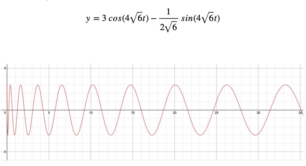
Applying a bit of intuition to this graph shows that over time the frequency of the oscillations begin to decrease, that is to say a lower frequency. However, since this is an undamped spring system notice that the amplitude never decreases. That is the spring system has the ability to restore all of its energy in compression and elongation.

Video Lesson:

https://www.dropbox.com/s/4q5klxo489chygu/RPReplay_Final1606190322.MP4?dl=0

Project #3


Section 6.3, Question 3

Find the current (I) in the RLC circuit, assuming that E(t) = 0 for t>0.

R = 2 ohms, L = 0.1 henrys, C = 0.01 farads,$ Q_o$ = 2 coulombs, $I_o$ = 0 amperes

According to Kirchhoff’s Law the sum of the voltage drops in a closed RLC circuit is equal to the impressed voltage E(t).

L$I’$ + RI + $\frac{1}{C}$Q = E(t)

This equation can be rewritten by replacing I with Q’ because charge stored in a capacitor is related to the current according to the equation below:

Q = $Q_o$ + $\int_{0}^{t}$ I($\tau$) d$\tau$

Rewritten Equation:

L$Q”$ + R$Q’$ + $\frac{1}{C}$ = E(t)

Substituting the values of L, R, C, and E(t) we get:

0.1 $Q”$ + 2 $Q’$ + $\frac{1}{0.01}$ Q = 0

0.1 $Q”$ + 2 $Q’$ + 100 Q = 0

Characteristic Equation:

0.1 $r^2$ + 2r + 100 = 0

Use the quadratic formula to find roots.

r = $\frac{(-2)\pm\sqrt{2^2-4(0.1)(100)}}{2(0.1)}$

= $\frac{-2\pm\sqrt{-36}}{0.2}$

= $\frac{-2\pm6i}{0.2}$

r = $-10\pm30i$

$r_1$ = $-10 + 30i$, $r_2$ = $-10-30i$

Roots are complex so general solution is:

y=$e^{\lambda x}$[$C_1$cos($\omega x$) + $C_2$sin($\omega x$)]

$\lambda$ = (-10), $\omega$ = (30) based on the roots we found

so;

Q(t) = $e^{-10t}$[$C_1$cos(30t)+$C_2$sin(30t)]

with $Q_o$=Q(0)=2 coulombs when t=0 we can solve for constant $C_1$

Q(0)=$e^{-10(0)}$[$C_1$cos(30 $\times$ 0)+$C_2$sin(30 $\times$ 0)]

cos(0)=1, sin(0)=0

2 = 1[$C_1$$\times$1+0]

2 = $C_1$

$I_o$=0 amperes : $I_o$=$Q’_o$=0 we use this to solve for constant $C_2$ and t=0

Q(t) = $e^{-10t}$[$C_1$cos(30t)+$C_2$sin(30t)]

$\frac{d}{dt}$Q(t) = ($e^{-10t}$[$C_1$cos(30t)+$C_2$sin(30t)]) $\frac{d}{dt}$

$Q'(t)$=[-10$C_1$ $e^{-10t}$ cos(30t) – 30$C_1$ $e^{-10t}$ sin(30t)] + [-10$C_2$ $e^{-10t}$ sin(30t) + 30$C_2$ $e^{-10t}$ cos(30t)]

0 = [-10$\times$ 2 $e^{-10(0)}$ cos(30$ \times 0$) – 30 $\times$ 2 $e^{-10(0)}$ sin(30$\times$ 0)] + [-10$C_2$ $e^{-10(0)}$ sin(30$\times$ 0) + 30$C_2$ $e^{-10(0)}$ cos(30$\times$ 0)]

0 = -20 + 0 + 0 + 30$C_2$

20 = 30$C_2$

$\frac{2}{3}$ = $C_2$

Therefore:

Q(t) = 2$e^{-10t}$cos(30t) + $\frac{2}{3}$ $e^{-10t}$sin(30t)

We differentiate Q(t) to get the current (I).

$\frac{d}{dt}$Q(t) = [2$e^{-10t}$cos(30t) + $\frac{2}{3}$ $e^{-10t}$sin(30t)]$\frac{d}{dt}$

$Q'(t)$ = I = -20$e^{-10t}$cos(30t) – 60$e^{-10t}$sin(30t) – $\frac{20}{3}$ $e^{-10t}$sin(30t) + 20$e^{-10t}$cos(30t)

I = $\frac{-200}{3}$ $e^{-10t}$sin(30t)

Project#3: Section 6.3: Problem 6

Video

(click the link to view video)

https://www.dropbox.com/s/zz4kf2w0p2j8mzh/Enriquez_MAT2680_Project_3.MOV?dl=0

Pictures

Steps

Use “Undetermined coefficients” method

  1. Solve for the roots of the characteristic equation.
    • use quadratic formula
    • use the the roots of the characteristic equation to find the solution of the complimentary equation
      • refer back to solutions of “constant coefficient second order linear equations”
  2. Find a suitable general form for a “particular solution”, $y_{p}$ , that matches the “right side of the given equation” ($y_{p}$ is the same as $Q_{p}$, which is function representing the amount of charge of a sytem).
    • if the right side of the equation is $cos(ct)$, $sin(ct)$, or $cos(ct)+sin(ct)$, then the particular solution is of the form $Acos(ct)+Bsin(ct)$
    • since no terms in $y_{p}$ is a solution of the complimentary equation, no extra steps are necessary in deciding the form of the particular solution
  3. Differentiate the chosen particular solution twice to find $y_{p}^’$ and $y_{p}^”$.
  4. Substitute the values of $y_{p}$ , $y_{p}^’$ , and $y_{p}^”$ into $Q$, $Q’$, and $Q”$.
  5. Simplify the new equation.
  6. Rearrange the terms of the equation (factoring may be necessary) so that the “left side of the equation” matches the form of the “right side of the equation”.
  7. Create and solve a system of equations to solve for the undetermined coefficients.
  8. Plug in the values of the undetermined coefficients into the chosen particular solution to determine $Q_{p}$.
  9. Since the steady steady state current, $I_{p}$ , is equal to $Q_{p}^’$ , we must differentiate $Q_{p}$ to solve for the steady state current of the system.
« Older posts