Contents
Video
(click the link to view video)
https://www.dropbox.com/s/zz4kf2w0p2j8mzh/Enriquez_MAT2680_Project_3.MOV?dl=0
Pictures
Steps
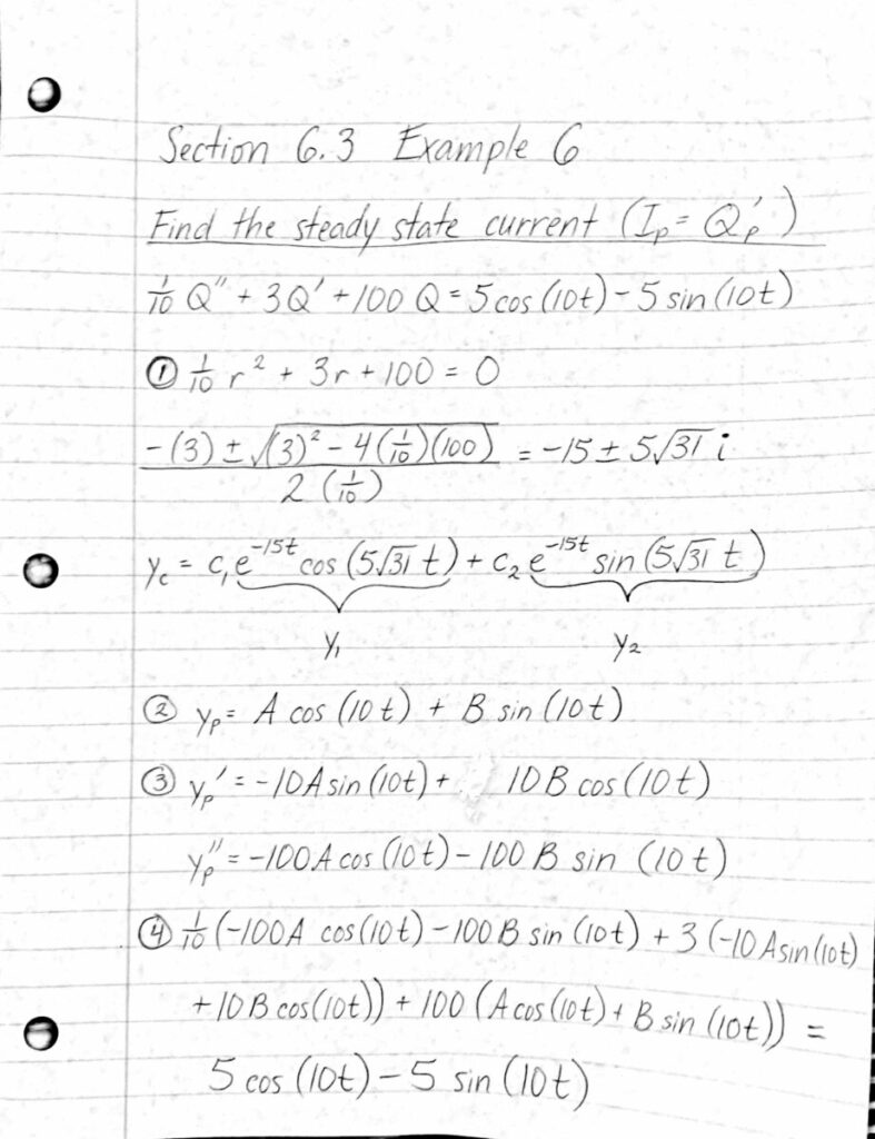
Use “Undetermined coefficients” method
- Solve for the roots of the characteristic equation.
- use quadratic formula
- use the the roots of the characteristic equation to find the solution of the complimentary equation
- refer back to solutions of “constant coefficient second order linear equations”
- Find a suitable general form for a “particular solution”, $y_{p}$ , that matches the “right side of the given equation” ($y_{p}$ is the same as $Q_{p}$, which is function representing the amount of charge of a sytem).
- if the right side of the equation is $cos(ct)$, $sin(ct)$, or $cos(ct)+sin(ct)$, then the particular solution is of the form $Acos(ct)+Bsin(ct)$
- since no terms in $y_{p}$ is a solution of the complimentary equation, no extra steps are necessary in deciding the form of the particular solution
- Differentiate the chosen particular solution twice to find $y_{p}^’$ and $y_{p}^”$.
- Substitute the values of $y_{p}$ , $y_{p}^’$ , and $y_{p}^”$ into $Q$, $Q’$, and $Q”$.
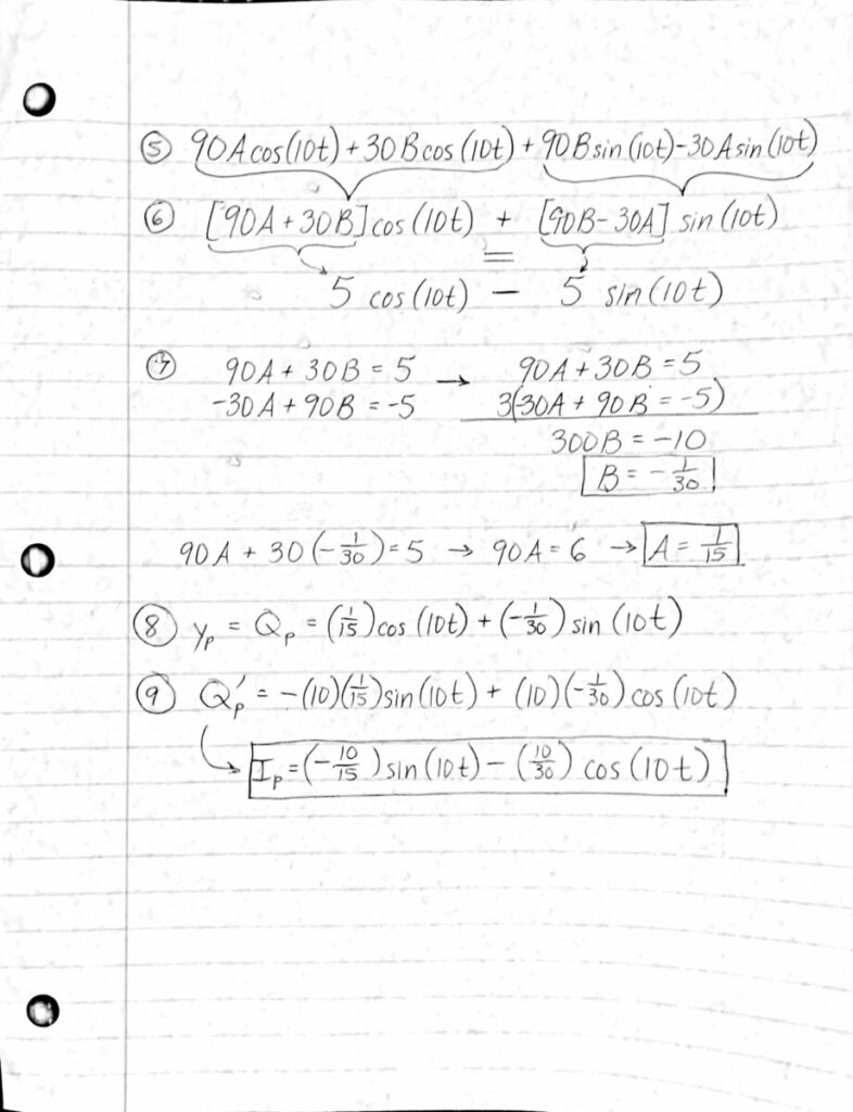
- Simplify the new equation.
- Rearrange the terms of the equation (factoring may be necessary) so that the “left side of the equation” matches the form of the “right side of the equation”.
- Create and solve a system of equations to solve for the undetermined coefficients.
- Plug in the values of the undetermined coefficients into the chosen particular solution to determine $Q_{p}$.
- Since the steady steady state current, $I_{p}$ , is equal to $Q_{p}^’$ , we must differentiate $Q_{p}$ to solve for the steady state current of the system.


Leave a Reply