Professor Kate Poirier | OL67 | Fall 2020

Category: Uncategorized (Page 1 of 5)

Project 4: The Differential Equations of Counter-Insurgencies

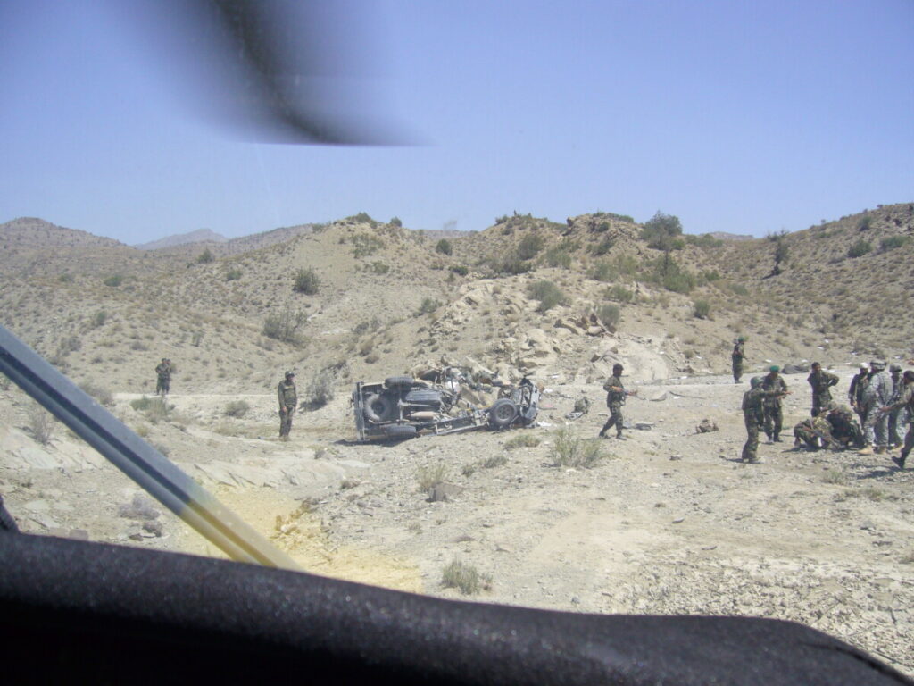
As a retired US Army Officer I have spent a good part of my adult life in the counter-insurgency business. Operationally we spent a lot of time analyzing the “Three Pillars” of counter-insurgency (often abbreviated as COIN) operations, they are, or were at one point: Security, Political and Economic. Over the course of my time spent in Afghanistan and Iraq I was mostly engaged in the Security and Economic “pillars”.

Basic terms of counter-insurgencies:

The Occupying Force: This would be the newly established, or emplaced, government.

The Insurgents: These are the people that are sympathetic to the old government or regime and are opposed to the new government. The insurgents do not have the military or economic power to reclaim control of government and therefore are only able to disrupt the operation of the new government or regime.

So with the foundations for the concept being well established I dove into the equations which are based on Lotka-Volterra equations often used to describe the interactions between two competing systems.

Here the numbers of occupiers are \begin{math}\omega(t)\end{math} and the number of insurgents are \begin{math}i(t)\end{math}. These ultimately represent the solutions for the problems. That is, what are the populations on each side of the insurgency or counter-insurgency after taking into account some influencing parameters.

eq 1:

\begin{math}\frac{di}{dt}\:=\: (a+d\omega-ei)i-Fi\omega \end{math}

Note: The interaction of \begin{math}-Fi\omega\end{math}, if this interaction is negative then the equation is modeling the Insurgent population. If the interaction sign is positive it will be modeling the Occupying Force.

where:

Recruitment of new insurgents: \begin{math}a\end{math}

Measure of the anger and motivation of the insurgents: \begin{math}d\end{math}

Actions of the Occupying Force to reduce the number of insurgents: \begin{math}F\end{math}

population of Insurgents: \begin{math}-ei\end{math}

eq 2:

\begin{math}\frac{d\omega}{dt}\:=\: r(C-\omega)i \end{math}

The second equation shows the relationship between the populations of insurgents and occupiers, specifically that the number of occupiers tends to increase as long as there is an active insurgent population, there is however a limit to the maximum size of the occupiers.

The maximum size the the occupying forces may achieve is:\begin{math}C>0\end{math}

The reaction of the occupiers to increase their force strength is: \begin{math}r\end{math}

When computed these equations seem to confirm with real world events and also seem to generally overlap with results from predator prey differential equations. Where the predator is similar to the occupying force and the prey are the insurgents.

I can see where using these equations could help drive decisions at various levels of foreign policy as well as giving ground commanders an idea of how to focus their resources in COIN operations.

References:

https://www.trinitydc.edu/wp-content/uploads/2016/01/Modeling-Interaction-of-Insurgency-and-Counterinsurgency-by-Differential-Equations-Chiang-2012..pdf

http://www.idea.wsu.edu/Insurgency/

https://www.math.utk.edu/~heather/231Project_Insurgencies.pdf

Project #3: Groups: Chapter 6.3: The RLC Circuit

6.3 The RLC Circuit

Introduction: 

The main purpose of chapter 6.3 is to show how differential equations can be used to solve RLC Circuits problems. RLC circuits can simply be explained as electrical circuits that consist of a resistor, an inductor, and a capacitor all connected to each other. Now to understand the real world problem part of this chapter, the function of the components must be understood. The resistor has many uses, in an electrical circuit one of its main purposes is to reduce current flow. The inductor protects the circuit from changes in the current that can damage other components. Finally the capacitor stores electric charges that can be denoted as (Q) which can be used for other purposes. In other words differences in potential occur at the resistor, induction coil, and the capacitor. RLC circuits have many applications that range from oscillator circuits to radio receivers.

 Now in chapter 6.3 we are mainly concerned with the difference in electric potential that occurs in a closed circuit, which is caused by the flow of a current in the circuit. In other words we are interested in the changes that occur in a RLC circuit when voltage(E) is introduced to the circuit producing a current(I) that runs across the circuit, and all the other components (R), (L), (C) finally giving us the electrical potential(E(t)). Now that we know what exactly we want to find out in the real world problem. This section is solving RLC circuit problems through the use of Linear Second Order Equations. In the following part of this lesson will be showing the ways in which all the units relate to each other and what formulas are used to solve the RLC problems.

In the image above we have an example of an RLC circuit and all the units need it to solve the RLC circuit problems. 
The following notations are used:
E= E(t)  for the electric potential/impressed voltage from a battery or generator 
I=I(t) for the current of the circuit
R is the resistance of the resistor
L is the inductance of the inductor
C is the capacitance of the capacitor 

In accordance with Kirchhoff’s Law, it is stated that the sum of the voltage drops in a closed RLC circuit equals the impressed voltage. Using formulas 1,2,4  from the section above we get the new formula:

Same as in Second Order Linear Equation problems there are also initial value problems.

In the example section several example problems are able to explain how these equations are solved.

Finally we also have Non-homogeneous Second Linear Equation Problems

This problem deals with forced oscillation with damping, a more thorough explanation is given in example 5 where a Non-homogeneous Second Linear Equation problem is explained and solved with the “undetermined coefficients” method.

Examples of RLC Circuit Problems:

Example 1:

Find the current in the RLC circuit, assuming that E(t) = 0

for t > 0.

R = 3 ohms; L = 0.1 henrys; C = 0.01 farads; Q0 = 0 coulombs; I0 = 2 amperes.

The video example and Solution is here.

Example 2:

Find the current in the RLC circuit, assuming that E(t) = 0

for t > 0.

R = 2 ohms; L = 0.05 henrys; C = 0.01 farads’; Q0 = 2 coulombs; I0 = 2 amperes.

The video example and Solution is here.

Example 3:

Find the current in the RLC circuit, assuming that E(t) = 0

for t > 0.

R = 2 ohms; L = 0.1 henrys; C = 0.01 farads; Q0 = 2 coulombs; I0 = 0 amperes.

Example 4:

Find the steady state current in the circuit describe by the equation.

1/10Q”+6Q’+250Q = 10 cos 100t + 30 sin100t

The video example and solution is here.

Find the steady state current in the circuit describe by the equation.

1/10Q”+3Q’+100Q = 5cos 10t – 5sin 10t

The video example and Solution is here.

« Older posts