Professor Kate Poirier | OL67 | Fall 2020

Category: Project #3 (Page 2 of 5)

Project #3


Section 6.3, Question 3

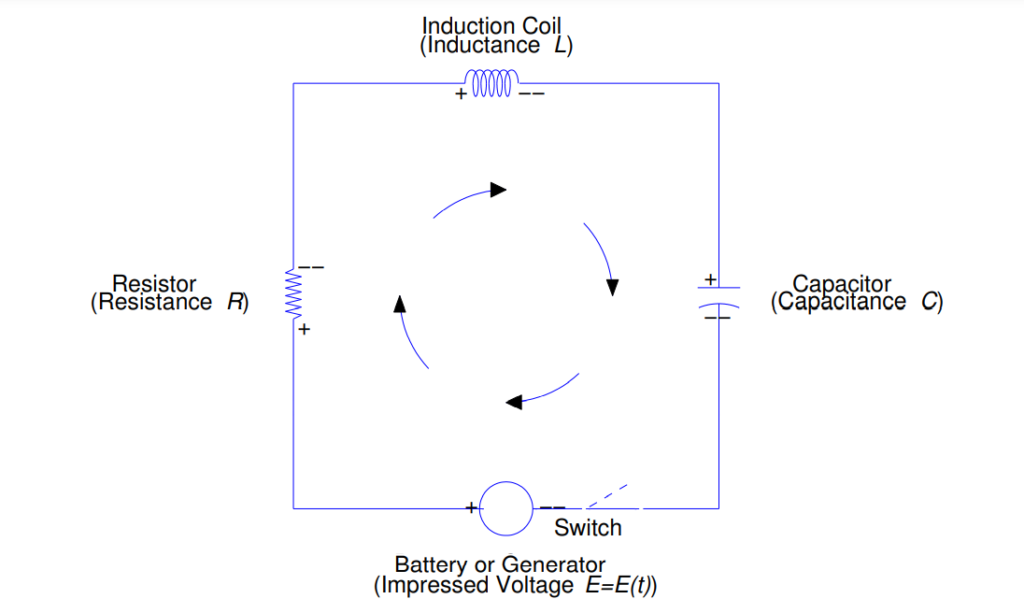
Find the current (I) in the RLC circuit, assuming that E(t) = 0 for t>0.

R = 2 ohms, L = 0.1 henrys, C = 0.01 farads,$ Q_o$ = 2 coulombs, $I_o$ = 0 amperes

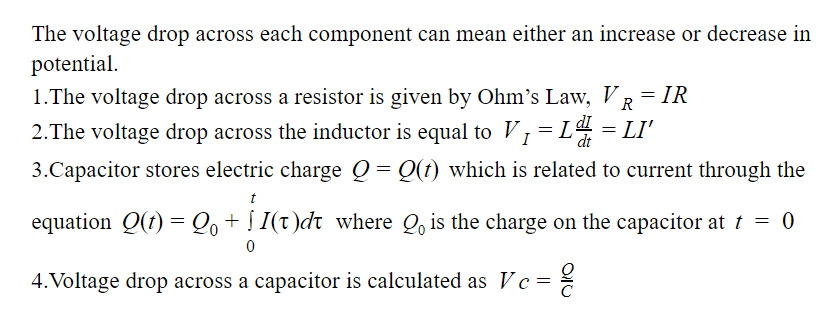
According to Kirchhoff’s Law the sum of the voltage drops in a closed RLC circuit is equal to the impressed voltage E(t).

L$I’$ + RI + $\frac{1}{C}$Q = E(t)

This equation can be rewritten by replacing I with Q’ because charge stored in a capacitor is related to the current according to the equation below:

Q = $Q_o$ + $\int_{0}^{t}$ I($\tau$) d$\tau$
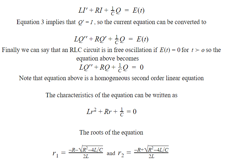
Rewritten Equation:

L$Q”$ + R$Q’$ + $\frac{1}{C}$ = E(t)

Substituting the values of L, R, C, and E(t) we get:

0.1 $Q”$ + 2 $Q’$ + $\frac{1}{0.01}$ Q = 0

0.1 $Q”$ + 2 $Q’$ + 100 Q = 0

Characteristic Equation:

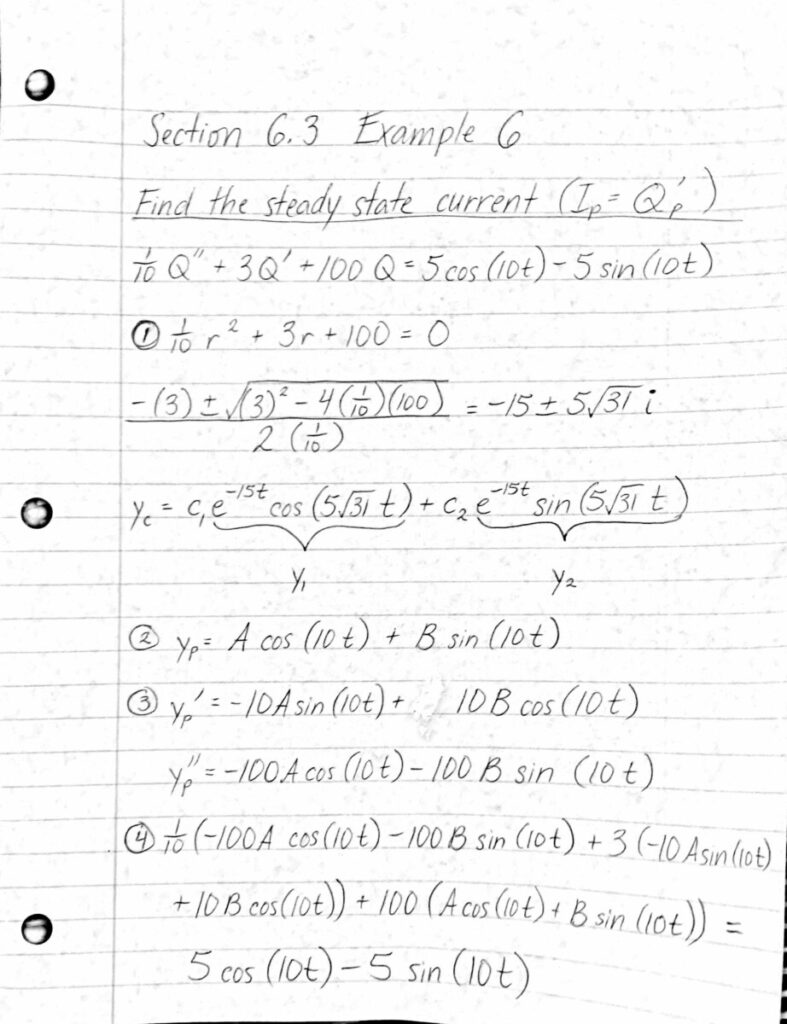
0.1 $r^2$ + 2r + 100 = 0

Use the quadratic formula to find roots.

r = $\frac{(-2)\pm\sqrt{2^2-4(0.1)(100)}}{2(0.1)}$

= $\frac{-2\pm\sqrt{-36}}{0.2}$

= $\frac{-2\pm6i}{0.2}$

r = $-10\pm30i$

$r_1$ = $-10 + 30i$, $r_2$ = $-10-30i$

Roots are complex so general solution is:

y=$e^{\lambda x}$[$C_1$cos($\omega x$) + $C_2$sin($\omega x$)]

$\lambda$ = (-10), $\omega$ = (30) based on the roots we found

so;

Q(t) = $e^{-10t}$[$C_1$cos(30t)+$C_2$sin(30t)]

with $Q_o$=Q(0)=2 coulombs when t=0 we can solve for constant $C_1$

Q(0)=$e^{-10(0)}$[$C_1$cos(30 $\times$ 0)+$C_2$sin(30 $\times$ 0)]

cos(0)=1, sin(0)=0

2 = 1[$C_1$$\times$1+0]

2 = $C_1$

$I_o$=0 amperes : $I_o$=$Q’_o$=0 we use this to solve for constant $C_2$ and t=0

Q(t) = $e^{-10t}$[$C_1$cos(30t)+$C_2$sin(30t)]

$\frac{d}{dt}$Q(t) = ($e^{-10t}$[$C_1$cos(30t)+$C_2$sin(30t)]) $\frac{d}{dt}$

$Q'(t)$=[-10$C_1$ $e^{-10t}$ cos(30t) – 30$C_1$ $e^{-10t}$ sin(30t)] + [-10$C_2$ $e^{-10t}$ sin(30t) + 30$C_2$ $e^{-10t}$ cos(30t)]

0 = [-10$\times$ 2 $e^{-10(0)}$ cos(30$ \times 0$) – 30 $\times$ 2 $e^{-10(0)}$ sin(30$\times$ 0)] + [-10$C_2$ $e^{-10(0)}$ sin(30$\times$ 0) + 30$C_2$ $e^{-10(0)}$ cos(30$\times$ 0)]

0 = -20 + 0 + 0 + 30$C_2$

20 = 30$C_2$

$\frac{2}{3}$ = $C_2$

Therefore:

Q(t) = 2$e^{-10t}$cos(30t) + $\frac{2}{3}$ $e^{-10t}$sin(30t)

We differentiate Q(t) to get the current (I).

$\frac{d}{dt}$Q(t) = [2$e^{-10t}$cos(30t) + $\frac{2}{3}$ $e^{-10t}$sin(30t)]$\frac{d}{dt}$

$Q'(t)$ = I = -20$e^{-10t}$cos(30t) – 60$e^{-10t}$sin(30t) – $\frac{20}{3}$ $e^{-10t}$sin(30t) + 20$e^{-10t}$cos(30t)

I = $\frac{-200}{3}$ $e^{-10t}$sin(30t)

Project #3: Groups: Chapter 6.3: The RLC Circuit

6.3 The RLC Circuit

Introduction: 

The main purpose of chapter 6.3 is to show how differential equations can be used to solve RLC Circuits problems. RLC circuits can simply be explained as electrical circuits that consist of a resistor, an inductor, and a capacitor all connected to each other. Now to understand the real world problem part of this chapter, the function of the components must be understood. The resistor has many uses, in an electrical circuit one of its main purposes is to reduce current flow. The inductor protects the circuit from changes in the current that can damage other components. Finally the capacitor stores electric charges that can be denoted as (Q) which can be used for other purposes. In other words differences in potential occur at the resistor, induction coil, and the capacitor. RLC circuits have many applications that range from oscillator circuits to radio receivers.

 Now in chapter 6.3 we are mainly concerned with the difference in electric potential that occurs in a closed circuit, which is caused by the flow of a current in the circuit. In other words we are interested in the changes that occur in a RLC circuit when voltage(E) is introduced to the circuit producing a current(I) that runs across the circuit, and all the other components (R), (L), (C) finally giving us the electrical potential(E(t)). Now that we know what exactly we want to find out in the real world problem. This section is solving RLC circuit problems through the use of Linear Second Order Equations. In the following part of this lesson will be showing the ways in which all the units relate to each other and what formulas are used to solve the RLC problems.

In the image above we have an example of an RLC circuit and all the units need it to solve the RLC circuit problems. 
The following notations are used:
E= E(t)  for the electric potential/impressed voltage from a battery or generator 
I=I(t) for the current of the circuit
R is the resistance of the resistor
L is the inductance of the inductor
C is the capacitance of the capacitor 

In accordance with Kirchhoff’s Law, it is stated that the sum of the voltage drops in a closed RLC circuit equals the impressed voltage. Using formulas 1,2,4  from the section above we get the new formula:

Same as in Second Order Linear Equation problems there are also initial value problems.

In the example section several example problems are able to explain how these equations are solved.

Finally we also have Non-homogeneous Second Linear Equation Problems

This problem deals with forced oscillation with damping, a more thorough explanation is given in example 5 where a Non-homogeneous Second Linear Equation problem is explained and solved with the “undetermined coefficients” method.

Examples of RLC Circuit Problems:

Example 1:

Find the current in the RLC circuit, assuming that E(t) = 0

for t > 0.

R = 3 ohms; L = 0.1 henrys; C = 0.01 farads; Q0 = 0 coulombs; I0 = 2 amperes.

The video example and Solution is here.

Example 2:

Find the current in the RLC circuit, assuming that E(t) = 0

for t > 0.

R = 2 ohms; L = 0.05 henrys; C = 0.01 farads’; Q0 = 2 coulombs; I0 = 2 amperes.

The video example and Solution is here.

Example 3:

Find the current in the RLC circuit, assuming that E(t) = 0

for t > 0.

R = 2 ohms; L = 0.1 henrys; C = 0.01 farads; Q0 = 2 coulombs; I0 = 0 amperes.

Example 4:

Find the steady state current in the circuit describe by the equation.

1/10Q”+6Q’+250Q = 10 cos 100t + 30 sin100t

The video example and solution is here.

Find the steady state current in the circuit describe by the equation.

1/10Q”+3Q’+100Q = 5cos 10t – 5sin 10t

The video example and Solution is here.

Project#3: Section 6.3: Problem 6

Video

(click the link to view video)

https://www.dropbox.com/s/zz4kf2w0p2j8mzh/Enriquez_MAT2680_Project_3.MOV?dl=0

Pictures

Steps

Use “Undetermined coefficients” method

  1. Solve for the roots of the characteristic equation.
    • use quadratic formula
    • use the the roots of the characteristic equation to find the solution of the complimentary equation
      • refer back to solutions of “constant coefficient second order linear equations”
  2. Find a suitable general form for a “particular solution”, $y_{p}$ , that matches the “right side of the given equation” ($y_{p}$ is the same as $Q_{p}$, which is function representing the amount of charge of a sytem).
    • if the right side of the equation is $cos(ct)$, $sin(ct)$, or $cos(ct)+sin(ct)$, then the particular solution is of the form $Acos(ct)+Bsin(ct)$
    • since no terms in $y_{p}$ is a solution of the complimentary equation, no extra steps are necessary in deciding the form of the particular solution
  3. Differentiate the chosen particular solution twice to find $y_{p}^’$ and $y_{p}^”$.
  4. Substitute the values of $y_{p}$ , $y_{p}^’$ , and $y_{p}^”$ into $Q$, $Q’$, and $Q”$.
  5. Simplify the new equation.
  6. Rearrange the terms of the equation (factoring may be necessary) so that the “left side of the equation” matches the form of the “right side of the equation”.
  7. Create and solve a system of equations to solve for the undetermined coefficients.
  8. Plug in the values of the undetermined coefficients into the chosen particular solution to determine $Q_{p}$.
  9. Since the steady steady state current, $I_{p}$ , is equal to $Q_{p}^’$ , we must differentiate $Q_{p}$ to solve for the steady state current of the system.
« Older posts Newer posts »