Enzyme kinetics of Turnip Peroxidase

Hydrogen peroxide (H₂O₂) is a strong oxidizing agent that can damage cells and is formed as a by-product of oxygen consumption. Fortunately, aerobic cells contain peroxidases that break down peroxide into water and oxygen. This enzyme reduces hydrogen peroxide into H₂O by oxidizing an organic compound (AH₂ -> A).

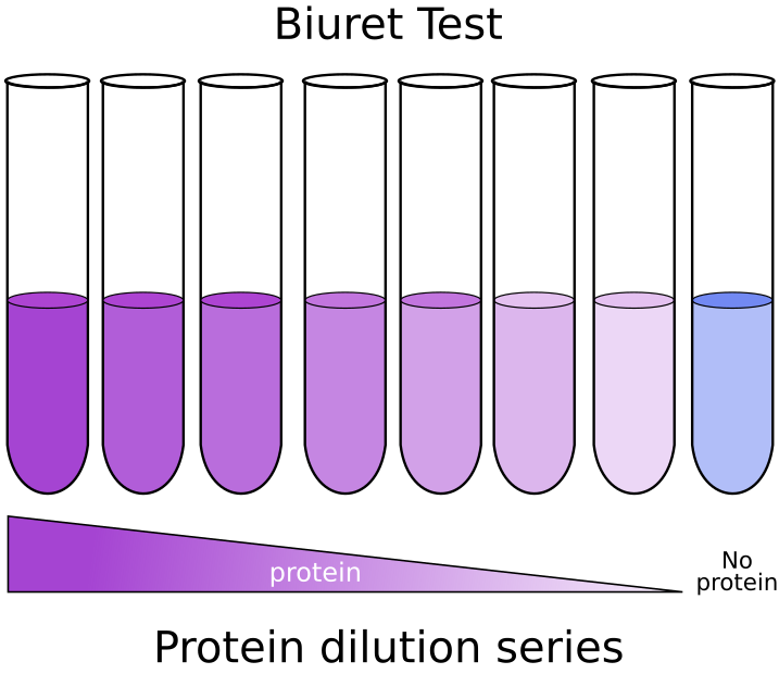
This exercise uses turnip extract as a source of peroxidase. This turnip extract requires a source of electrons (a reducing agent) in order for the reaction to occur. In this case, a colorless organic compound called guaiacol is used. Guaiacol is oxidized in the process of converting the peroxide and becomes brown. Enzymatic activity can then be traced using a spectrophotometer to measure the amount of brown being formed.

Hypotheses on Enzyme Kinetics

Use the following questions to develop your hypotheses based on the background understanding of enzymes. Discuss if the outcomes matched your hypotheses following these exercises

1. What effect does pH have on the rate of enzyme activity? Explain this with respect to the nature of enzymes.
2. Predict the optimal pH for turnip peroxidase activity.
3. What influence do you think a cold temperature (ice bucket or 0-4ºC) would have on the rate of the turnip peroxidase activity?
4. What influence do you think a warm temperature (around human body temperature or fever 37-40ºC) would have on the rate of turnip peroxidase activity?
5. What outcome can you predict of the rates when changing the concentration of enzyme or substrate?

Set-up and Calibrate SpectroVis Plus

1. Plug SpectroVis to computer via USB cable
2. Launch Vernier Spectral Analysis (https://www.vernier.com/product/spectral-analysis/)
3. Begin a new experiment by choosing “Absorbance vs. Time (Kinetics)”
4. Wait for Lamp to warm up if necessary
5. Place a blank cuvette in the unit and press “Finish Calibration”
6. Enter a wavelength of 500nm and press “done”
7. Proceed to the individual exercises

 

Effect of pH on Peroxidase Activity

1. Set-up cuvette for pH 3
   1. Add 10 drops 0.02% hydrogen peroxide
   2. Add 5 drops 0.2% guaiacol
   3. Add 20 drops of pH 3 buffer
   4. Add 10 drops turnip extraction last
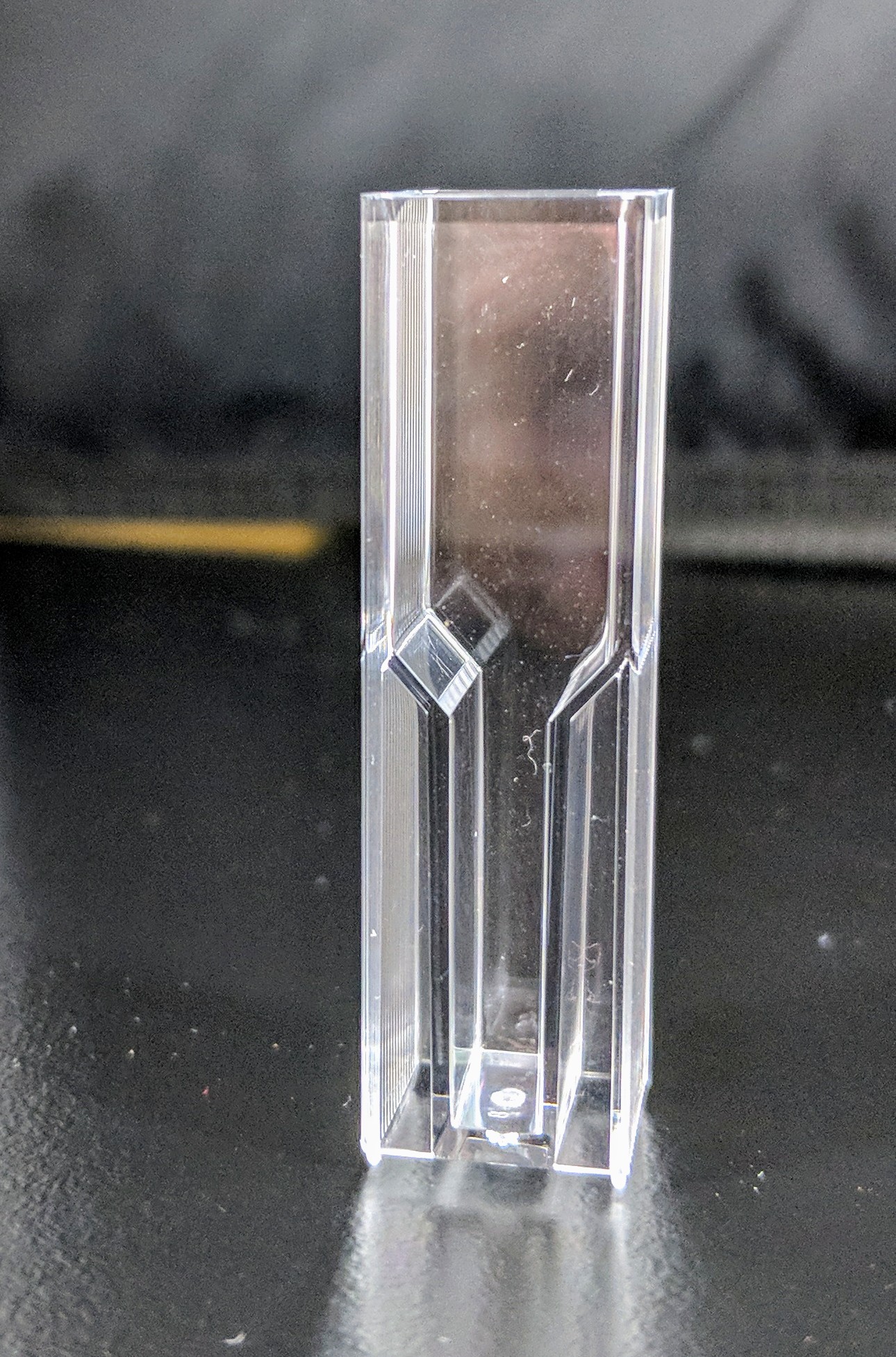
   5. Quickly invert the cuvette to mix and place the upright cuvette into the Spectrovis Plus
   6. Press “Collect” to begin recording data
      1. 1. Stop data collection after 200s
         2. “Export Data” as a “.csv” file to computer or a USB flash drive
            • Ensure that it has saved as a “.csv” file
            • this will open in a text editor or spreadsheet
2. Sequentially repeat the experiment exchanging the pH buffer with pH 5, 7, 10

Effect of Temperature on Peroxidase Activity

1. Buffers are incubated on ice (0ºC), at room temperature (20ºC), in 40ºC or 60ºC at least 5 minutes
2. Set-up cuvette for 0ºC
   1. Add 10 drops 0.02% hydrogen peroxide (incubated at 0ºC for 10 minutes)
   2. Add 5 drops 0.2% guaiacol
   3. Add 20 drops of extraction buffer at 0ºC
   4. Add 10 drops turnip extraction (incubated at 0ºC for 10 minutes) last
   5. Quickly invert the cuvette to mix and place the upright cuvette into the Spectrovis Plus
   6. Press “Collect” to begin recording data
      1. Stop data collection after 200s
      2. “Export Data” as a “.csv” file to computer or a USB flash drive
         • Ensure that it has saved as a “.csv” file
         • this will open in a text editor or spreadsheet
3. Sequentially repeat the experiment exchanging the buffers stored at 20ºC, 40ºC, 60ºC

 Effect of Substrate Concentration on Peroxidase Activity

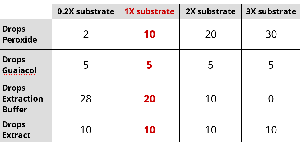
1. Set-up cuvette for 1X substrate
   1. Add 10 drops 0.02% hydrogen peroxide
   2. Add 5 drops 0.2% guaiacol
   3. Add 20 drops of extraction buffer
   4. Add 10 drops turnip extraction last
   5. Quickly invert the cuvette to mix and place the upright cuvette into the Spectrovis Plus
   6. Press “Collect” to begin recording data
      1. 1. Stop data collection after 200s
         2. “Export Data” as a “.csv” file to computer or a USB flash drive
            • Ensure that it has saved as a “.csv” file
            • this will open in a text editor or spreadsheet
2. Sequentially repeat the experiment with differing amounts of buffer and peroxide:
   1. 1. Repeat the experiment with 0.2X substrate and export data to USB drive
      2. Repeat the experiment with 2X substrate and export data to USB drive
      3. Repeat the experiment with 3X substrate and export data to USB drive

 

 Effect of Enzyme Concentration on Peroxidase Activity

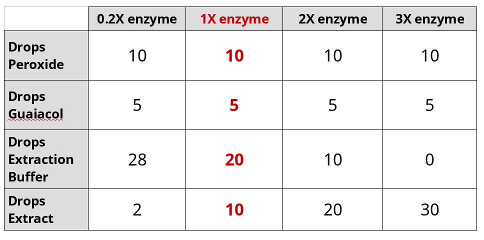
1. Set-up cuvette for 1X enzyme
   1. Add 10 drops 0.02% hydrogen peroxide
   2. Add 5 drops 0.2% guaiacol
   3. Add 20 drops of extraction buffer
   4. Add 10 drops turnip extraction last
   5. Quickly invert the cuvette to mix and place the upright cuvette into the Spectrovis Plus
   6. Press “Collect” to begin recording data
      1. 1. Stop data collection after 200s
         2. “Export Data” as a “.csv” file to computer or a USB flash drive
            • Ensure that it has saved as a “.csv” file
            • this will open in a text editor or spreadsheet
2. Sequentially repeat the experiment with differing amounts of buffer and extract:
   1. 1. Perform the experiment on 1X enzyme and export data to USB drive
      2. Repeat the experiment with 0.2X enzyme and export data to USB drive
      3. Repeat the experiment with 2X enzyme and export data to USB drive
      4. Repeat the experiment with 3X enzyme and export data to USB drive

 

Tags: quantitative reasoning

Hardy-Weinberg Principle

The Hardy-Weinberg principle is a mathematical model used to describe the equilibrium of two alleles in a population in the absence of evolutionary forces. This model was derived independently by G.H. Hardy and Wilhelm Weinberg. It states that the allele and genotype frequencies across a population will remain constant across generations in the absence of evolutionary forces. This equilibrium makes several assumptions in order to be true:

1. An infinitely large population size
2. The organism involved is diploid
3. The organism only reproduces sexually
4. There are no overlapping generations
5. Mating is random
6. Allele frequencies equal in both genders
7. Absence of migration, mutation or selection

As we can see, many items in the list above can not be controlled for but it allows for us to make a comparison in situations where expected evolutionary forces come into play (selection etc.).

Hardy-Weinberg Equilibrium

The alleles in the equation are defined as the following:

• Genotype frequency is calculated by the following:
• Allele frequency is calculated by the following:
• In a two allele system with dominant/recessive, we designate the frequency of one as p and the other as q and standardize to:
  • 
  • 
• Therefore the total frequency of all alleles in this system equal 100% (or 1)
  • 
• Likewise, the total frequency of all genotypes is expressed by the following quadratic where it also equals 1:
  • 
  • This equation is the Hardy-Weinberg theorem that states that there are no evolutionary forces at play that are altering the gene frequencies.

Calculating Hardy-Weinberg Equilibrium (activity)

This exercise refers to the PTC tasting exercise. One can test for selection for one  allele within the population using this example. Though the class size is small, pooling results from multiple section can enhance the exercise. Remember to surmise the dominant/recessive traits from the class counts.

1. What is the recessive phenotype and how can we represent the genotype?
2. What is the dominant phenotype and how can we represent the genotypes?
3. What is the frequency of recessive genotype? (q²)
4. What is the frequency of the recessive allele? (q)
5. What is the frequency of the dominant allele?(p=1-q)
6. Use Hardy-Weinberg to calculate the frequency of heterozygotes in the class. (2pq)
7. Use Hardy-Weinberg to calculate the frequency of homozygotes in the class. (p²)
8. Using an aggregate of multiple section, compare the local allelic and genotypic frequencies with what the Hardy-Weinberg would predict.
9. With this small number in mind, we can see that there are problems with the assumptions required for this principle. The instructor will perform the following simulation in class to illustrate the effects on multiple populations with the effects of selection and /or population limitations. A coefficient of fitness can be applied to illustrate a selective pressure against an allele.
   • Population Genetics Simulation of Alleles
10. In the case of a selective pressure, a fitness coefficient (w) can be introduced. A research article http://www.jci.org/articles/view/64240 has shown that the Tas2R38 receptor aids in the immune response against Pseudomonas. Imagine a situation where there is an epidemic of antibiotic resistant Pseudomonas. This would
    show that the dominant allele will have a selective advantage.
    • Modify the fitness coefficient in the Population Genetics Simulator and describe the effects this would have over many successive generations.

A case study of evolution: Population Genetics at Work

Additional Resources/Experiments

• Population Genetics Simulation of Alleles (Schaffer)
• Population Genetics Simulation of Alleles (Sheehy)
•  Lee RJ, Xiong G, Kofonow JM, Chen B, Lysenko A, Jiang P, Abraham V, Doghramji L, Adappa ND, Palmer JN, Kennedy DW, Beauchamp GK, Doulias PT,Ischiropoulos H, Kreindler JL, Reed DR, Cohen NA. T2R38 taste receptor polymorphisms underlie susceptibility to upper respiratory infection. J Clin Invest. 2012;122(11):4145-4159. doi:10.1172/JCI64240.

 

 

Tags: quantitative reasoning, integration of knowledge

Mendel’s Observations

Probability: Past Punnett Squares

Punnett Squares are convenient for predicting the outcome of monhybrid or dihybrid crosses. The expectation of two heterozygous parents is 3:1 in a single trait cross or 9:3:3:1 in a two-trait cross. Performing a three or four trait cross becomes very messy. In these instances, it is better to follow the rules of probability. Probability is the chance that and event will occur expressed as a fraction or percentage. In the case of a monohybrid cross, 3:1 ratio means that there is a 3/4 (0.75) chance of the dominant phenotype with a 1/4 (0.25) chance of a recessive phenotype.

 

A single die has a 1 in 6 chance of being a specific value. In this case, there is a 1/6 probability of rolling a 3. It is understood that rolling a second die simultaneously is not influenced by the first and is therefore independent. This second die also has a 1/6  chance of being a 3.

We can understand these rules of probability by applying them to the dihybrid cross and realizing we come to the same outcome as the 2 monohybrid Punnett Squares as with the single dihybrid Punnett Square.

This forked line method of calculating probability of offspring with various genotypes and phenotypes can be scaled and applied to more characteristics.

Tags: quantitative reasoning, integration of knowledge, guided inquiry

Quantitative PCR (qPCR)

Measurements can be made of individual genes of interest through PCR of those specific genes. A process known as Real-Time PCR or quantitative PCR (qPCR) is used to measure individual genes using fluorescence measurements. An intercalating agent that binds only to double stranded DNA called Sybr Green is used in a qPCR machine that is measuring fluorescence after each cycle of PCR indirectly indicates the amount of amplified product. However, non-specific products of amplification may also be measured and not discriminated from the authentic amplicon.

An alternative to Sybr Green is exemplified by the TaqMan technology. With TaqMan, a third primer (TaqMan probe) is designed in the middle of the area to be amplified. This middle primer is designed with a hairpin self-complimentarity so that the 5′ and 3′ ends are in close proximity. At one end, a fluorescent reporter is attached while the other terminus has a quencher that absorbs any fluorescence signal. Under normal circumstances, measurements of fluorescence will be very low. When PCR extension occurs, the Polymerase hydrolyzes this middle primer, thereby separating the quencher and reporter. The name TaqMan is a play on words since it is imagined that the polymerase is chewing up the probe like Pacman. With increased distance between quencher/reporter, fluorescence signal from this probe can now be measured. This method is much more specific than Sybr Green, however the use of specific probes increases the cost considerably.

Threshold Cycles (C_t)

Fluorescence measurement early during the PCR process will be very low due to small number of dsDNA molecules (Sybr Green) or most TaqMan primers being quenched. During this exponential DNA production, a threshold will be reached in which the fluorescence will linearly increase. A specific point where the fluorescence is clearly measurable called the Threshold Cycle (C_t) is used as a reference point to compare expression values.

Looking at the example of Sybr Green qPCR above, it can be observed that samples exponentially increasing at a lower Cycle number (C_t) has a higher level of mRNA expression (towards the left) of that gene than samples with higher cycle number (towards the right). Notice that the fluorescence eventually plateaus and stops increasing. This is due to the depletion of raw materials for DNA production like dNTPs.

Since the PCR reactions theoretically represent a doubling of DNA after each cycle, the C_t values can be interpreted on a base 2 system. If there is a difference in C_t between two samples (ΔC_t) of 5 cycles, this corresponds to 2⁵ or 32 fold difference. We can control for variations in the RNA preparation through comparing the fluorescence values of our gene of interest to a housekeeping gene like actin. The use of a house-keeping gene to normalize the initial input to the reactions and comparison between samples is referred to as Relative Quantification.

Melt Curves for Sybr Green

When using Sybr Green, we need to ensure that the PCR is specific so that the fluorescence measurement truly reflect amplification of our gene of interest. At the end of each qPCR run (~40 cycles), a melt curve is performed. A melting curve (or dissociation curve) comes from constant measurements as the temperature is increased. As temperature increases, the DNA strands start to denature and fluorescence will begin to decrease. After complete separation of DNA strands, the fluorescence will again remain constant. The way this curve is viewed is through a derivative plot where the inflection in fluorescence reading is reported as the melting temperature (Tm).

Any peaks in this plot refer to a specific PCR product. If multiple peaks appear, the results will not be valid as they do not directly measure a single product.

Expression measurements

Differential gene expression refers to transcriptional programs activated by the cell under various conditions. “Differential” refers to a comparison of two or more states or timepoints. Using mRNA as an indirect measurement of protein, one can ascertain which proteins are linked to these different states. In eukaryotes, this can be assessed by enriching total RNA for polyA-containing mature mRNA. Through the use of oligo-(dT) containing resin, mRNA can be separated from non-protein encoding RNA. Likewise, performing a reverse-transcription using an oligo-(dT) primer will create a stable complimentary DNA (cDNA) molecule that can be used with PCR. Using qPCR in this way is called RT-PCR or reverse-transcription polymerase chain reaction where specific primer pairs are used to amplify a small portion of a known gene.

Hybridization based methods and Microarrays

Prior to RT-PCR, expression of individual genes was assessed through a hybridization-based approach. This method called for running RNA on an agarose gel and transferring the size-fractionated RNAs onto a membrane through a method called “blotting”. This transferred RNA was then hybridized to a radioactively labelled probe for a specific gene (corresponding to the reverse complimentary sequence) and visualized by exposure to X-ray film in a process called Northern Blotting. The intensity of the band would be proportional to the amount of mRNA corresponding to the gene of interest. Re-probing with a housekeeping gene like actin would be used as a loading control to illustrate that a similar amount of total RNA was loaded into each well. Differences in sizes of the mRNA on the Northern Blot also revealed differences in splice variants of mature mRNA in the different states.

This technique was later adapted using non-radioactive methods. Using these non-radioactive methods, the reverse protocol was developed to measure multiple gene targets. By systematically immobilizing gene specific probes onto a membrane or a microscope slide, an array of targets can be produced. In the simplest paradigm of having 2 states (control or experimental), cDNA from each sample can be used to generate fluorescent RNA that can hybridize to immobilized probes. Using 2 different fluorescent markers allows for the competitive hybridization onto the array whereby the fluorescent signal in each channel can reveal the differential gene expression of the two states in a 2-color microarray.

Detection and measuring amount of a virus by RT-PCR

COVID-19 is a disease caused by SARS-CoV2 virus. This virus is characterized as a (+) ss-RNA virus with a genome of about 30kb.

In order to detect this virus, respiratory tract samples are collected and the RNA extracts are subjected to reverse transcription followed by PCR of a portion of the N gene. The exponential nature of PCR permits for the detection of the complementary DNA in minuscule concentrations. By using standards of known concentrations, quantitative PCR (qPCR) effectively determine the viral load within the cells.

The following video demonstrates the lab work involved in titrating Adeno-Associated Virus (AAV) by qPCR. While AAV has a genome of ssDNA, this video illustrates similar steps in quantitation.

 

Tags: quantitative reasoning, integration of knowledge

Morphometrics and physical markers

Morphometrics (morpho– shape; metrics– measurements) is the use of physical measurements to determine the relatedness of organisms. With extinct organisms that have died out long ago, DNA extraction proves to be difficult. Likewise, prior to DNA technologies to analyze species, Linnean taxonomy was ascribed to organisms based on similarities in features.

Describing Species and Variation of Morphologies

Below are images of skull landmarks of the lizard family Varanidae. This family includes monitor lizards and Komodo Dragons.As can be seen below, the general morphology of the skulls are similar enough that they all retain the same landmarks. The figure below also illustrates the diversity in these lizards that illustrate a large variety between species.

Landmarks Standardize measurements

Having a set of shared landmarks provides the opportunity to make systematic measurements of morphometric features.

 

Euclidean distance to measure relatedness

Euclidean distance is a measurement derived from Pythagorean geometry that describes the shortest distance (d) between 2 points (A & B) as a straight line using triangulation. In a cartesian space, the points can be defined:

and 

Standard pythagorean theorem can be expressed as:

To find the distance between the 2 points, we utilize algebra to calculate for .

In this case, we expand to comparing the coordinates of the two points:

and

We can then expand this idea to include the differences of data points that describe the comparisons of multiple measurements.

Calculating distance with R

1. Download the dataset (McCurry et al. 2015) associated with this activity (a Comma Separated Value .csv file). This can be used in a spreadsheet or in a text editor. This data can be imported into R to determine the euclidean distances of landmarks.
2. The following code in R will download the data set into a variable called “varanoid”, measure euclidean distance and save a plot into a PDF file in a directory called “/tmp”.

## install curl for fetching from internet if it isn't
install.packages('curl')
## Load the curl library
library(curl)
## read the data of measurements and assign it to a variable 'varanoid'
varanoid = read.csv(curl('https://raw.githubusercontent.com/jeremyseto/bio-oer/master/data/varanoid.csv'))
## set the row names to the Species column
row.names(varanoid) = varanoid$Species
## remove the first column of the table to have purely numeric data
varanoid_truncated = (varanoid[,2:14])
## calculate distance using euclidean as the method
dist_measure = dist(varanoid_truncated, method='euclidean')
## display dist_measure to look at the comparisons
dist_measure
varanoid_cluster = hclust(dist_measure)
## open PDF as a graphics device  to save a file in the '/tmp' directory
pdf(file='/tmp/varanoid_tree.pdf')
plot(varanoid_cluster)
dev.off()
## close the device to save the plot as pdf

 

 

DNA Analysis

Before starting this activity, review bioinformatics and sequence analysis.

1. Search NCBI for mitochondrial sequences from the species involved in McCurry 2015. The data has been submitted by Ast (2001).
2. Find the sequences and identify/extract elements that are common to all
3. Assemble the shared sequences in a text editor as a single FASTA file where each species is separated by a header (“>Species A”)
   • Notepad on Windows (but it’s better to download notepad++)
   • Textedit on Mac (but probably better to download TextWrangler)
   • Gedit on Linux
4. Save the file as “something.fasta”
5. Perform a multiple sequence analysis using UGENE
6. Generate a phylogenetic tree using UGENE. For this exercise, use Maximum Likelihood (PhyML) as the algorithm. File the tutorial below.
7. Compare the DNA with the morphometric analyses. What problems could we imagine arise if we rely solely on morphometry.

References

• McCurry MR, Mahony M, Clausen PD, Quayle MR, Walmsley CW, Jessop TS, Wroe S, Richards H, McHenry CR. (2015) The Relationship between Cranial Structure, Biomechanical Performance and Ecological Diversity in Varanoid Lizards. PLoS ONE 10(6): e0130625. doi: 10.1371/journal.pone.0130625
• Ast, Jennifer C. (2001) Mitochondrial DNA Evidence and Evolution in Varanoidea (Squamata). Cladistics 17(3): 211–26.  http://www.sciencedirect.com/science/article/pii/S0748300701901690
• Fisher, R.A. (1936) The use of multiple measurements in taxonomic problems.  Annals of Eugenics, 7: 179–188. doi:10.1111/j.1469-1809.1936.tb02137.x

Tags: quantitative reasoning, analysis, visual communication, integration of knowledge, breadth of knowledge

Prelab Exercise

1. Fill the Color field in the table below
2. Use plot.ly to create a line graph with the 3 samples below (A, B, C)
   • plot % Reflectance on the Y-axis and Wavelength (nm)  on the X-axis

		% Reflectance
Color	nm	A	B	C
	400	68	92	78
	425	40	71	77
	450	90	38	51
	475	97	49	57
	500	100	92	45
	525	100	100	66
	550	96	97	100
	575	98	96	100
	600	96	98	100
	625	97	80	100
	650	79	71	100
	675	56	96	100
	700	88	100	100

Stop and Think: Reflectance

A sign of plant health is viewed through the near infra-red. While we cannot see this spectrum of light with our eyes, we can use other sensors to detect this light. Compare the images of the Black & White with the Infra-red image. What differences can you see in the 2 images that will help you understand how this is a useful measure of plant health? How do you think this is corresponds to the table above?

Reflectance Slider shows an overlay of the next images

Visible light wavelengths (between 400nm-700nm) are strongly absorbed by the pigments in leaves (Chlorophylls, Xanthophylls, Carotenoids). These pigments utilize the energy of these wavelengths to take part in the light reactions. The cellular structure of leaves do not absorb wavelengths longer than these wavelengths (>700nm in the infra-red range). By comparing the amount of visible light to the amount of near infra-red light that are reflected, one can gauge the relative health of leaves, forests or jungles . This is the rough description of the Normalized Differential Vegetation Index (NDVI) that scientists use in conjunction with satellite imagery to assess the health of vegetation.

The Role of Light in Carbohydrate Synthesis

1. Pick a leaf from a geranium exposed to light and one kept in the dark for 48 hours.
   • keep the stem on the leaf grown in light
   • remove the stem from the leaf grown in the dark
2. Hydrolyze the cell walls of the geranium leaves by boiling in a water bath for 5 minutes or until it looks like over-cooked vegetables)
3. “Bleach“ the leaves by  removing the pigments. Place the leaves in hot alcohol for 7 minutes or until they turn white.
   1. Save this green solution for Absorbance Spectrum exercise
4. Remove the leaves and place it in a petri dish.
5. Add iodine to the dish. If starch is present, the leaf will turn a deep bluish-black color.
6. Photograph the leaf with your phone to document the effects of light on carbohydrate storage.

Measuring Absorbance

1. Connect the Spectrovis to the Computer via USB
2. Launch Vernier Spectral Analysis software
3. Open a new experiment and choose “Full Spectrum”
4. Press OK to calibrate
5. Let the machine calibrate for 90 seconds
6. Choose “Finish calibration”
7. Insert the Geranium pigment from the bleaching reaction
   1. Do NOT use Acetone in these plastic cuvettes since it will frost over the plastic
8. Press the Red Stop button
9. Students should export the experiment as a csv file
10. The professor will prepare Spirulina extract diluted in ethanol in a cuvette and obtain the continuous absorbance spectrum.
11. Plot Relative Absorbance against wavelength using a line graph and compare the absorption spectrum of the extracts.
    1. Relative Absorbance sets the maximum value in each dataset as a denominator
    2. Every value is divided by this maximum value
    3. Plot these points using Chart Studio/Plot.ly with Relative Absorbance as a function of Wavelength

Tags: quantitative reasoning

Extract and separate the pigments

1. Lay a strip of filter paper on the bench
2. about 2 cm from the bottom of the strip, place a fresh spinach leaf and rub a coin across the leaf to transfer pigment to the strip
3. The instructor will be provided with a spoonful of Spirulina powder that has been soaked in 10ml acetone overnight.
   • on a separate strip, the instructor will apply the Spirulina extract approximately 2cm from the bottom of the strip
4. Suspend the strips by a dowel or paper clip in a tube with about 3ml chromatography solution (2 isooctane: 1 acetone: 1 diethyl ether).
5. Develop the strips until the solvent reaches about 2 cm from the top

Chromatography Analysis

1. How many different pigments separate from the spinach extract? From the spirulina?
2. Are all pigments represented between the two extract?
3. The mobile phase is non-polar, what are the properties of each pigment?
4. Measure the R_f of each pigment.

Tags: quantitative reasoning

The Enzyme

Amylase is an enzyme that breaks down amylose (starch) into glucose molecules.

1. 1. 1. What test can be used to indicate the presence of Starch?
      2. What test can be used to indicate the presence of glucose?
      3. What is the role of an enzyme in a chemical reaction and what is it made of?
      4. What parameters would influence the ability of the enzyme to facilitate the rate of the reaction?

Tags: quantitative reasoning, analysis, inquiry, integration of knowledge

Experimental Background

Bovine Serum Albumin (BSA) is a protein that circulates in the blood of cows. Purified BSA can be used with Biuret solution in serial dilutions to generate a Standard Curve. The standard curve will illustrate the relationship between concentration (the dependent variable) and absorbance at 540 nm (the independent variable).  We can then use this curve to estimate the concentration of unknown samples.

1. On a graph, do you remember which axis is the dependent and which is the independent variable?
2. In the table below, can you identify which samples are the negative controls and which are the positive controls?
3. What is the prediction of the absorbance or color intensity of the different tubes?

Dilute BSA Standards

1. Label 9 tubes A-I
2. Combine the components of the table below to generate appropriate concentration of solutions

3. The instructor will provide 2 unknown samples to each group
   1. Connect SpectroVis Plus to computer via USB
   2. Launch the Vernier Spectral Analysis program or Chrome App
   3. Select “By Concentration (Beer’s Law)”
   4. Unit will warm up the lamp
   5. After warm-up has completed, place a blank cuvette into the SpectroVis and select “Calibrate”
   6. Select Wavelength to 540nm and press “Done”
   7. In the data table, click on “…”  and change units to “mg/ml”
4. Place sample in the SpectroVis and press “Collect”
   1. After the absorbance value has stabilized, press “Keep”
   2. Enter  the concentration of the sample solution
   3. Press “Keep Point”
5. Replace with a new sample solution and start from step 4 (“Collect”) for each new solution
6. Do NOT press “Keep” when reading the absorbance of the unknown solutions.
   1. 1. simply record those absorbance values manually
7. Sequentially read each sample at the stored wavelength (A_540nm)and record values in table below

1. Plot each BSA dilution in plot.ly as a scatterplot (Log-on using Facebook/Google/Twitter credentials for free)
2. Generate best-fit line for these standards with the equation of the line
3. Use the equation of the line to estimate the concentration of the unknown sample.

Distance Learning Simulation Exercise

• https://docs.google.com/document/d/1UMoPkqSXNUW70VglxhCQvA_Dj7hlgkG-qmcOrbv6jUc/edit?usp=sharing

Curve Fitting

Review: https://openlab.citytech.cuny.edu/bio-oer/biology-basics/quantitative-skills/

Run the simulation below to understand how you can use the standard dilution series to estimate your sample concentrations.

Scatterplot Tutorial

You can watch this tutorial at 1.25X and pause when needed.

Tags: quantitative reasoning

Course Presentation: https://h5p.org/node/280305

Energy and catalysts

In Biological systems, energy is roughly defined as the capacity to do work. Molecules are held together by electrons. Breaking and building these bonds requires an input of energy. The energy needed to initiate such reactions is referred to as activation energy (E_A). Sometimes the necessary energy to initiate a reaction is so great, that it greatly limits the likelihood of the reaction ever occurring. Catalysts are chemicals that take part in facilitating reactions by reducing the energy of activation. If the activation energy is reduced, the likelihood of a reaction occurring is greatly enhanced. In cells, the catalysts are often made of proteins and called enzymes.

Enzymes

Reactants in enzymatic reactions are called substrates. They have an imperfect fit to a binding domain of the enzyme called the active site. Substrate binding to this active site induces a change in the shape of the protein that coordinates the substrate into a transition state that will reduce the amount of E_A required for the reaction to go to completion. The induced fit of the protein also aids in coordinating other cofactors or coenzymes that will aid in the reaction.

 

The reaction follows the standard flow where the Enzyme (E) and the Substrate (S) interact to form an Enzyme-Substrate Complex (ES). The ES then dissociates into Enzyme and the resultant Product (P)

E + S ⇒ ES ⇒ E + P

The induced fit of the enzyme-substrate complex coordinates the transition state to facilitate the reaction. This induced fit occurs through non-covalent means that result in a tugging on the molecules (an application of energy) while molecules are coaxed into the reactions.

Coenzymes can be covalently linked to amino acid side chains of the enzyme and are also referred to as prosthetic groups. While prosthetic groups are organic in nature, they may also involve the coordination of metal ions, like the heme group which binds to iron. These prosthetic groups enhance the repertoire of the amino acids to provide additional functioning to the entire protein. Early coenzymes were described as being vital to normal functioning and were characterized as organic molecules with amine groups. Because of this coincidence, they were referred to as vitamins (for vital amines) though not all vitamins have amine groups. The trace metal ions that work with these groups are also required and represent the minerals on food items.

Tags: quantitative reasoning, visual communication, integration of knowledge