A linear differential equation is called homogeneous if the following condition is satisfied: If is a solution, so is , where is an arbitrary (non-zero) constant. Note that in order for this condition to hold, each term in a linear differential equation of the dependent variable y must contain y or any derivative of y.
A separable differential equation is any differential equation that we can write in the following form.
Note that in order for a differential equation to be separable all the y‘s in the differential equation must be multiplied by the derivative and all the x‘s in the differential equation must be on the other side of the equal sign. Solving separable differential equation is fairly easy. We first rewrite the differential equation as the following
Then you integrate both sides.
Example
Example 2: Solve the equation
This equation is separable, since the variables can be separated:
The integral of the left‐hand side of this last equation is simply
and the integral of the right‐hand side is evaluated using integration by parts:
The solution of the differential equation is therefore
In mathematics, an integrating factor is a function that is chosen to facilitate the solving of a given equation involving differentials. It is commonly used to solve ordinary differential equations, but is also used within multivariable calculus when multiplying through by an integrating factor allows an inexact differential to be made into an exact differential (which can then be integrated to give a scalar field). This is especially useful in thermodynamics where temperature becomes the integrating factor that makes entropy an exact differential.
Consider an ordinary differential equation that we wish to solve to find out how the variable y depends on the variable x. If the equation is first order then the highest derivative involved is a first derivative. If it is also a linear equation then this means that each term can involve y either as the derivative OR through a single factor of y. Any such linear first order can be re-arranged to give the following standard form:
dy/dx + P(x)y = Q(x); Where P(x) and Q(x) are functions of x, and in some cases may be constants.
A linear first order o.d.e. can be solved using the integrating factor method. After writing the equation in standard form, P(x) can be identified. One then multiplies the equation by the following “integrating factor”:
IF= e^integral (P (x)dx )
This factor is defined so that the equation becomes equivalent to:
d/dx (IF y) = IF Q(x),
Whereby integrating both sides with respect to x, gives:
IF y = Integral (IF Q(x) dx)
Finally, division by the integrating factor (IF) gives y explicitly in terms of x, i.e. gives the solution to the equation.
Here are some Videos of how the problems are solved.
This is my partner Robert Morels Part of the project:
Overview
What is Integrating factor? To sum it all up its bacially a function that is chosen to make easier to solve a given equation that has differentials included. Its usually used to answer differential equations. At first you may think the procedure is a bit odd but intill you get towards the end is when it can make more sense. examine an usual differential equation that we need to solve to find out how the variable y depends on the variable x. if we notice that the equation happens to be in first order then the highest derivative involved is a first derivative. Note that if its also a linear equation then this means that each term can involve y either as the derivative dy/dx OR through a single factor of y .
Example
An integrating factor is a function by which an ordinary differential equation can be multiplied in order to make it integrable. We begin to spot when it can be used. We begin with starting from a standard form of ordinary differential equation.
(dy)/(dx)+f(x)y=q(x),
Once we get our equation we can jot down that f(x) and g(x) are two random functions of x only. When handling equations like this you must know that this form isn’t separable BUT we can join together the two terms on the left side into a single differential by using an integrating factor.
First we compute the integrating factor IF which is given to us by integrating f(x) then expanding the answer:
IF=e^f(x)
Now we defined F(x)=f(x)dx. When we integrate the function f(x) to get F9X) we don’t adda contstant. We are only focus in the function in the integrating factor F(X).
(dF/dx)=f(x)
This translate to the differential of the integrating factor:
(d/dx)e^F(x)=(dF/dx)x(e^F(x))=f(x)e^F(x)
Where we used the chain rule. We begin to multiply both side of the equation:
(e^F(x))(dy/dx)+f(x)e^F(x)y=g(x)e^F(x)
Here is where you may thing its getting pretty odd, but theres a reason for that is that the left hand side is now simply the differential of the integratinf factor multiplied by y:
d/dx(e^F(x)y)=(e^F(x))(dy/dx)+f(x)e^F(x)y
This now gives us a chance to write out the orginal equation in a simpler format:
d/dx(e^F(x)y)=g(x)e^F(x)
now we begin to integrate both sides
d/dx(e^F(x)y)dx=g(x)(e^F(x))dx
Integration is the opposite of differentiation, which makes it possible for the left side to cancel each other out, we then get the following:
e^F(x)y=g(x)(e^F(x))dx
if the integration on the right side is easy to compute this will lead towards our solution.
Videos
I included some videos that solve different equations using the method I provided above.
Video # 1:
Video #2:
In this pertectlar video the instructor is solving the following equation of
What is Integrating factor? To sum it all up its basically a function that is chosen to make easier to solve a given equation that has differentials included. It’s usually used to answer differential equations.. At first you may think the procedure is a bit odd but until you get towards the end is when it can make more sense. Examine a usual differential equation that we need to solve to find out how the variable y depends on the variable x. if we notice that the equation happens to be in first order then the highest derivative involved is a first derivative. Note that if it’s also a linear equation then this means that each term can involve y either as the derivative dy/dx OR through a single factor of y .
2. Example
An integrating factor is a function by which an ordinary differential equation can be multiplied in order to make it integral. We begin to spot when it can be used. We begin with starting from a standard form of ordinary differential equation.
(dy)/(dx)+f(x)y=q(x),
Once we get our equation we can jot down that f(x) and g(x) are two random functions of x only. When handling equations like this you must know that this form isn’t separable BUT we can join together the two terms on the left side into a single differential by using an integrating factor.
First we compute the integrating factor IF which is given to us by integrating f(x) then expanding the answer:
IF=e^f(x)
Now we defined F(x)=f(x)dx. When we integrate the function f(x) to get F9X) we don’t add a constant. We are only focus in the function in the integrating factor F(X).
(dF/dx)=f(x)
This translates to the differential of the integrating factor:
(d/dx)e^F(x)=(dF/dx)x(e^F(x))=f(x)e^F(x)
Where we used the chain rule. We begin to multiply both side of the equation:
(e^F(x))(dy/dx)+f(x)e^F(x)y=g(x)e^F(x)
Here is where you may thing its getting pretty odd, but there’s a reason for that is that the left hand side is now simply the differential of the integrating factor multiplied by y:
d/dx(e^F(x)y)=(e^F(x))(dy/dx)+f(x)e^F(x)y
This now gives us a chance to write out the original equation in a simpler format:
d/dx(e^F(x)y)=g(x)e^F(x)
Now we begin to integrate both sides
d/dx(e^F(x)y)dx=g(x)(e^F(x))dx
Integration is the opposite of differentiation, which makes it possible for the left side to cancel each other out, we then get the following:
e^F(x)y=g(x)(e^F(x))dx
if the integration on the right side is easy to compute this will lead towards our solution.
3. Videos
I included some videos that solve different equations using the method I provided above.
Video #2
In this particular video the instructor is solving the following equation of
In mathematics, an integrating factor is a function that is chosen to facilitate the solving of a given equation involving differentials. It is commonly used to solve ordinary differential equations, but is also used within multivariable calculus when multiplying through by an integrating factor allows an inexact differential to be made into an exact differential (which can then be integrated to give a scalar field). This is especially useful in thermodynamics where temperature becomes the integrating factor that makes entropy an exact differential.
Consider an ordinary differential equation that we wish to solve to find out how the variable y depends on the variable x. If the equation is first order then the highest derivative involved is a first derivative. If it is also a linear equation then this means that each term can involve y either as the derivative OR through a single factor of y. Any such linear first order can be re-arranged to give the following standard form:
dy/dx + P(x)y = Q(x);
Where P(x) and Q(x) are functions of x, and in some cases may be constants.
A linear first order o.d.e. can be solved using the integrating factor method. After writing the equation in standard form, P(x) can be identified. One then multiplies the equation by the following “integrating factor”:
IF= e^integral (P (x)dx )
This factor is defined so that the equation becomes equivalent to:
d/dx (IF y) = IF Q(x),
Whereby integrating both sides with respect to x, gives:
IF y = Integral (IF Q(x) dx)
Finally, division by the integrating factor (IF) gives y explicitly in terms of x, i.e. gives the solution to the equation.
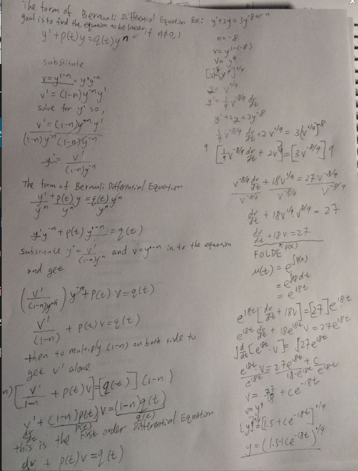
The form of Bernoulli Equations is y’+p(x) y=q(x)y^n, which n is just some real number. As we known that if n=1 or n=0 then after we plug it in to the n of the equation y’+p(x) y=q(x)y^n then we get y’+p(x) y=q(x)y^0 or y’+p(x) y=q(x)y^1. It shows you that it is just the first order linear differential equation that we already known how to solve it. However, if n ≠ 0, 1 then we need to use another method to solve it and it is called the Bernoulli equations. Here are the steps to solve the Bernoulli Differential Equations. In order to solve the Bernoulli Differential Equations as the first order linear differential equation first we need to set a) v=y^(1-n) and after we take the derivative of it we come up with b) v’= (1-n)y^(-n) y’.
We can get y’ alone by dividing by(1-n)y^(-n), and get y’=v’/((1-n) )*y^n. From the original Bernoulli Differential Equations y’+p(x) y=q(x)y^n. We can divided by y^n from the right side of the equation and get y^(-n) *[y]^’+y^(-n)*p(x)*y=q(x). Then we can substitute y’=v’/((1-n) )*y^n in to y’ in this equation y^(-n) 〖*y〗^’+y^(-n)*p(x) y=q(x) and gety^(-n) (v’/((1-n) ))*y^n+y^(1-n)*p(x) y=q(x), so we can cancel y^(-n) and y^n. We multiply (1-n) both side and get the First Order Differential equation v’ + (1-n)*p(x)*v= (1-n) =q(x)
Example:
y’+2y=3*y^(-8)
As we recognize that n≠1 or 0, so we need to use the Bernoulli Equations to transformed into a linear equation.
n=-8
put n=-8 in to the substitution of
v=y^(1-n)
v=y^(9)
we need to get y so, multiply the exponent 1/9 on each side and get
y=v^(1/9), then we take the derivative of it, and it becomes
y’=1/9*v^(-8/9)*(dv/dt)
after we get y’ and y then we can substitute in to the y’+2y=3*y^(-8) to solve for the linear equation
[1/9*v^(-8/9)*(dv/dt)]+[2v^(1/9)]=3(v^(-8/9))
then we multiply 1/9 on both side and divide by v^(-8/9), then we get
[dv/dt]+[18v]=27, and we recognize it is a First Order Linear Differential Equation dy/dx+p(x)y=f(x)
18 is p(x)
µ(t)=e^(∫p(x))
=e^(∫8dx)
=e^(18t)
we multiply e^(18t) of [dv/dt]+[18v]=27 and get
e^(18t)*[dv/dt]+e^(18t)*[18v]=e^(18t)*27
and take the integral on both side to get v alone so we can substitute y
∫d/dt[e^(18t)*v]=∫e^(18t)*27 and get
e^(18t)*v=27e^(18t)+c divide e^(18t) on both side
v=27/18+ce^(-18t)
we known that v=y^(9) from the beginning and plug it back to v
y^(9)=27/18+ce^(-18t), so we can multiply the exponent on both side by (1/9) and get the answer
y(t)=(1.5+ce^(-18t))^(1/9)
Here are the helpful videos that solve the Bernoulli equation step by step.
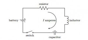
Electric circuits can consist of a wide variety of complex components. These may be set up in series, or in parallel, or even as combinations of both. However, we’ll be considering only series circuits with especially simple components: resistors, inductors, and capacitors, along with some form of voltage supply.
To start with, let’s consider the picture of a simple series circuit in which one of each of the components that we mentioned above appears:
L is a constant representing inductance, and is measured in Henry
R is a constant representing resistance, and is measured in ohms
C is a constant representing capacitance, and is measured in farads
E represents the electromotive force, and is measured in volts. It is not necessarily a constant, and may be a function of time
Let Q(t) be the charge in the capacitor at time t (Coulombs). Then dT /dt is called the current, denoted I. The battery produces a voltage (potential difference) resulting in current I when the switch is closed. The resistance R results in a voltage drop of RI. The coil of wire (inductor) produces a magnetic field resisting change in the current. The voltage drop created is L(dI/dt). The capacitor produces a voltage drop of Q/C. Unless R is too large, the capacitor will create sine and cosine solutions and, thus, an alternating flow of current. Kirchhoff Law states that “The sum of the voltage drops across each component in a circuit is equal to the voltage, E, impressed upon the circuit.” so
Restating Kirchhoff’s second law in abbreviated form, we get the following:
sum of the voltage drops = E,
which may be restated as:
inductor voltage drop + resistor voltage drop + capacitor voltage drop = E,
into which we may substitute the actual voltage drops that we mentioned above, to get:
(1)
LI′ + RI + q/C = E.
But, also according to physics, I = q′, so substituting, we can rewrite the equation purely in terms of the charge, q, rather than a mixture of charge and current:
(2)
Lq″ + Rq′ + q/C = E,
or alternatively, if we differentiate equation (1) and use the same substitution, we get an equation purely in terms of current:
(3)
L I″ + R I′ + I/C = E′.
We will be mainly concerned with using the last of these three equivalent forms.
Notice that equation (3) is linear with constant coefficients, so in this case when E′ = 0, (the homogeneous case), it may be solved very easily, even by hand.
The form of E′ will determine the method necessary when solving the non-homogeneous case by hand. We would need to use either undetermined coefficients, or variation of parameters.
An Example:
E(t) = 2e^t, R= 5Ω, C= 1/6 F, L= 1H
E(t)= Q`R + Q/R + Q/C + LQ“
=> 2e^t = Q`*5 + Q/(1/6) + L*Q“
=>2e^t = Q“ +5Q` + 6Q
r2 + 5r + 6 = 0
r2 + 3r + 2r + 6 =0
(r+3)(r+2) = 0
r = -3
r = -2
Q = Ae-3t + Be-2t
Guess:
Q = Ce^t
Q` = Ce^t
Q“ = Ce^t
Ce^t + 5Ce^t + 6 Ce^t = 2 e^t
12Ce^t = 2e^t
6Ce^t = e^t
C = 1/6
Q = Ae^(-3t) + Be^(-2t) + (1/6)e^t
Initial charge Q(0) = 11C
Initial Current I(0) = -18A
Take Q` and plug in
Q = Ae^(-3t) + Be^(-2t) + (1/6)e^t
Here are some videos which may also help to solve electrical Circuit in Differential Equation
What is Euler’s Method? Euler’s method is another way to solve differential equation problems in first order. Most first order differential equations however fall into none of the categories such as linear, separable, or exact differential equation or differential equation. How we solve first order differential equations is by knowing what we are looking for, if you are only looking for long term behavior of a solution you can always sketch a direction field.
What do we need?
Initial value y (a) = b
Differential equation = f (t, y)
The slope at the initial point à f (a, b)
Initial point (a, b)
The many points to choose how many steps = h, (h+1)
Find the value of y at t = c, find y(c).
Summary of Euler’s Method
In order to use Euler’s Method to generate a numerical solution to an initial value problem of the form:
y′ = f(x, y)
y (xo) = yo
We decide upon what interval, starting at the initial condition, we desire to find the solution. We chop this interval into small subdivisions of length h. Then, using the initial condition as our starting point, we generate the rest of the solution by using the iterative formulas:
xn+1 = xn + h
yn+1 = yn + h f (xn, yn)
to find the coordinates of the points in our numerical solution. We terminate this process when we have reached the right end of the desired interval.
Video
Sample Problem #1
Consider the initial value problem = 3-2t-.5y, y (0) =1. Find y (1)
Euler’s Method
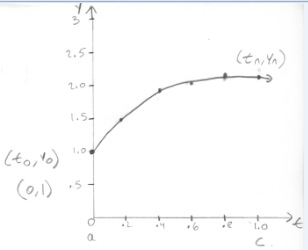
Approximate y by generating a series of points,
(t0, y0) = (a, b) = initial condition
(t1, y1)
(t2, y2)…
(tn, yn) = (c, yn), where yn is an approximation of y(c)
Goal: Find yn
Step size = h = (c-a)/n
h = (1-0)/5 = .2
t0 = 0
t1 = 0+.2 = .2
t2 = .2+.2 = .4
t3 = .4+.2 = .6
t4 = .6+.2 = .8
t5 = .8+.2 = 1
To go from one point (ti, yi) to the next (ti+1, yi+1)
Given the initial value problem y’ = sin (t +y +2), y (0) = 1.4, find approximate values of the solution at t = .7, t = 1.4 and t = 2.1, using Euler’s method with h = .7.
This is the beginning of a multi-part OpenLab assignment focussed on building resources for you and your fellow students. Our ultimate goal will be to create a study guide for this course, with videos and other resources for each topic.
Assignment (Due next Thursday, 3/26). Your first assignment is to choose a topic to work on. Fill in the form below, selecting THREE different topics that you would be interested in researching for our Study Guide (you will be assigned one of your three choices). Feel free to choose a topic that we have not yet studied (you will be given ample time to work on your portion of the Study Guide after we cover the topic in class).
You must be logged in to the OpenLab to complete this form. Having trouble with your account? Look here for help and resources: https://openlab.citytech.cuny.edu/2015-spring-mat-2680-reitz/?p=39
WolframAlpha, ridiculously powerful online calculator (but it doesn't do everything...) Slope Field Generator from Flash and Math Another Slope Field Generator That shows a specific solution for a given initial condition Desmos, completely awesome and free graphing calculator. The best for graphs! Sage Math Cloud, online access to heavyweight open source math applications (Sage, R, and more) - free registration required