Study Guide to Bernoulli Equations

Posted on April 30, 2015 by Compton Tudor | 1 comment

Overview

What are Bernoulli Equations?

Well to put it simply Bernoulli Equations are first order differential equations. What sets Bernoulli Equations apart from other first order differential equations is that they are nonlinear first order differential equation. When we was first introduced to first order differential equations we learned that the standard form was :

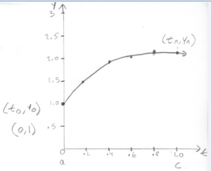
y’ +p(t)y = g(t) , y(to) = yo

What separates Bernoulli Equations from other first order equations is that in standard form, it is not equal to some function that is linear but one that has an exact solution. What this means is that their is some power that is raised to the right side of the equation which we shall call n and n cannot be equal to 0 or 1. this is what makes Bernoulli Equations nonlinear. Now we can change the form of a standard first order linear equation into a nonlinear first order equation:

y’ +p(t)y = q(t)y^(n) y(to)=yo

The above equation is now the standard form for a Bernoulli equation. What we can now understand from this equation is that p(t) and q(t) are functions that are continuous. Since n is a real number that has to be n> 0 and n>1 for this to be non linear.

Now the question is how do we solve Bernoulli Equations?

Sample Problem:

take an equation such as t^(2)y’ + 2ty – y^(3) = 0

and change it by adding y^(3) on both sides and we get:

t^(2)y’ + 2ty = y^(3)

Next we divide by t^(2) to on both sides of the equation so we can get it into standard form.

y’ + 2/yt = y^(3)/t^(2) <————-STANDARD FORM

Now we can go into the steps to solve this equation;

1. Divide by y^(n)

y’/y^(3) + 2/yt/y^(3) = (y^(3)/t^(2))/y^(3)

we get: (y’ + 2/yt)/y^(3) = 1/t^(2)

2. We substitute v = y^(1-n)

Since y^(3)

we get:v = y^(1-3) = y^(-2)

now we can rearrange the formula to so we can substitute v into it by moving the y^(2) to the numerator and we get:

y’/y^(3) + 2y^(-2)/t = 1/t^(2)

y’/y^(3) + 2v/t = 1/t^(2) <——————-Substitute v for y^(2)

Before we move to the solve Step we need to take the Derivative of the substitution v = y^(-2)

d/dy y^(-2)

dv/dt = -2y^(-3) dy/dt

(-1/2)v’ = -2y’/y^(3)(-1/2)

Now we can substitute for y’/y^(3) with the above equations and we get:

(-1/2)v’ + (2/t)v = 1/t^(2) <—————– First order linear equation

next we use the method of intergrating factor which states

mu = e^ intergral of (-4/t) which is equal to 1/t^(4)

we then multiply both sides b\by Mu and get the equation:

(dv(t)/dt)/t^(4) + d/dt(1/t^(4))v = (-2/t^(6))

Next we intergrate both sides and we come to the final answer of

y(t) = +- Sqrt(5t)/sqrt(ct^(5) + 2)

Videos:

I \\

1 Comment

Posted in Resources, Study Guide

Tagged advice for the future, divide by y^n, exact solutions, first order non linear, integrating factors, partial derivatives, standard form, substitute V=y^(1-n)

Electrical Circuits

Posted on April 29, 2015 by Anzamul Hyder | 1 comment

Electric circuits can consist of a wide variety of complex components. These may be set up in series, or in parallel, or even as combinations of both. However, we’ll be considering only series circuits with especially simple components: resistors, inductors, and capacitors, along with some form of voltage supply.

To start with, let’s consider the picture of a simple series circuit in which one of each of the components that we mentioned above appears:

L is a constant representing inductance, and is measured in Henry
R is a constant representing resistance, and is measured in ohms
C is a constant representing capacitance, and is measured in farads
E represents the electromotive force, and is measured in volts. It is not necessarily a constant, and may be a function of time

Let Q(t) be the charge in the capacitor at time t (Coulombs). Then dT /dt is called the current, denoted I. The battery produces a voltage (potential difference) resulting in current I when the switch is closed. The resistance R results in a voltage drop of RI. The coil of wire (inductor) produces a magnetic field resisting change in the current. The voltage drop created is L(dI/dt). The capacitor produces a voltage drop of Q/C. Unless R is too large, the capacitor will create sine and cosine solutions and, thus, an alternating flow of current. Kirchhoff Law states that “The sum of the voltage drops across each component in a circuit is equal to the voltage, E, impressed upon the circuit.” so

Restating Kirchhoff’s second law in abbreviated form, we get the following:

sum of the voltage drops = E,

which may be restated as:

inductor voltage drop + resistor voltage drop + capacitor voltage drop = E,

into which we may substitute the actual voltage drops that we mentioned above, to get:

(1)	LI′ + RI + q/C = E.

But, also according to physics, I = q′, so substituting, we can rewrite the equation purely in terms of the charge, q, rather than a mixture of charge and current:

(2)	Lq″ + Rq′ + q/C = E,

or alternatively, if we differentiate equation (1) and use the same substitution, we get an equation purely in terms of current:

(3)	L I″ + R I′ + I/C = E′.

We will be mainly concerned with using the last of these three equivalent forms.

Notice that equation (3) is linear with constant coefficients, so in this case when
E′ = 0, (the homogeneous case), it may be solved very easily, even by hand.

The form of E′ will determine the method necessary when solving the non-homogeneous case by hand. We would need to use either undetermined coefficients, or variation of parameters.

An Example:

E(t) = 2e^t, R= 5Ω, C= 1/6 F, L= 1H

E(t)= Q`R + Q/R + Q/C + LQ“

=> 2e^t = Q`*5 + Q/(1/6) + L*Q“

=>2e^t = Q“ +5Q` + 6Q

r2 + 5r + 6 = 0

r2 + 3r + 2r + 6 =0

(r+3)(r+2) = 0

r = -3

r = -2

Q = Ae-3t + Be-2t

Guess:

Q = Ce^t

Q` = Ce^t

Q“ = Ce^t

Ce^t + 5Ce^t + 6 Ce^t = 2 e^t

12Ce^t = 2e^t

6Ce^t = e^t

C = 1/6

Q = Ae^(-3t) + Be^(-2t) + (1/6)e^t

Initial charge Q(0) = 11C

Initial Current I(0) = -18A

Take Q` and plug in

Q = Ae^(-3t) + Be^(-2t) + (1/6)e^t

Here are some videos which may also help to solve electrical Circuit in Differential Equation

1 Comment

Posted in Uncategorized

Solving Repeated Roots

Posted on April 29, 2015 by Steven Ramlall | Leave a comment

Once you know how to solve second order linear homogeneous differential equations with constant coefficients, real or complex, the next step is to solve with those that have repeated roots. When solving for repeated roots, you could either factor the polynomial or use the quadratic equation, if the solution has a repeated root it means that the two solutions for “x” or whatever variable are the same.

Theorem for Solving Repeated Roots

Let: ay” + by’ + cy = 0

Be a differential equation such that the characterstic equation has the repeated root “r” That is :

(b^2)-4ac = 0

Then the general solution to the differential equation is given by

y = c₁e^rt + c₂te^rt

Leave a comment

Posted in Study Guide

Tagged advice for the future, differential equations repeated roots, Repeated Roots

Non-homogeneous Equation; Method of Undetermined Coefficients

Posted on April 29, 2015 by Rana Das | 6 comments

Title

Non-homogeneous Equation; Method of Undetermined Coefficients

Overview

The topic is about Non-homogeneous equation, with method of undetermined Coefficients. For our better understanding we all should know what homogeneous equation is. Homogeneous equation is a differential equation, which is equal to zero. However, before we proceed to solve the Non-homogeneous equation, with method of undetermined Coefficients, we must look for some key factors into our differential equation. For example, the differential equations must be linear and should not be more than second order. The method of undetermined coefficients is a use full technique determining a particular solution to a differential equation with linear constant-Coefficient.

Theorem

The form of the nonhomogeneous second-order differential equation, looks like this y”+p(t)y’+q(t)y=g(t) Where p, q and g are given continuous function on an open interval I. On the other hand, the homogenous part will look like, y’’+p(t)y’+q(t)y=0

Sample problem

A Sample Problem of Non-homogeneous Equation; Method of Undetermined Coefficients below:

y” – 4y’+ 3y= – 168e^7t , particular solution satisfying y(0)= 9 and y’(0)= -15.

Step 1:

Make this differential as a homogeneous differential equation
y” – 4y’+ 3y= 0	Note: The differential equation is now homogenous

Step 2:

Now we can write the homogenous differential to a characteristic equation.
r² – 4r + 3 = 0	Note: The differential equation is now characteristic polynomial.

Step 3:

Solve the characteristic equation
r² – 4r + 3 = 0r² – 3r – r +3 = 0r ( r -3 ) – 1 (r – 3)=0 (r – 3) ( r -1)=0		Note: 3 and 1 are the roots of the characteristic polynomial. After we find the roots of the polynomial, the Y₁ and Y₂ will take form of e^at. However, there are some exceptions and we will address it later ( at the end of the page )
(r – 3)=0 r= 3	( r -1)=0 Or r = 1
Y₁ = e^3t	Y_{2 =}e^t
y(t)= C₁ e^3t+ C₂ e^t		Note: This is homogeneous part of solution. Where C1 and C₂are the arbitrary constants.

Step 4:

Guessing Table
If the right side g(t)	We will guess
Ae^7t	Ce^7t
Example: – 168e^7t	Ce^7t Note: C is for arbitrary constants and e^7tis from the differential equation.
A sin(t)	C sin (t) + D Cos (t)
A cos (t)	C sin (t) + D Cos (t)
t²+ 7	Ct² + Dt + E

Step 5:

After appropriate guessing, now, we can process to solve the Non-homogeneous part of differential equation. Now we have to take the first and second derivative guess.

Guess:

Y(t) = Ce^7t

^y’= C (7e^7t)

y’’= C (49e^7t)

Then plug in the y(t), y’(t) and y’’(t) into the original differential equation. In this case, we will plug it into y” – 4y’+ 3y= – 168e^7t.

Non-homogeneous part of differential equation

y” – 4y’+ 3y= – 168e^7t

C (49e^7t) – C (4*7e^7t) + C (3e^7t)= – 168e^7t

C =(- 168e7t)/(24e7t)

C = -7e^7t

Note: Non-homogeneous solution to differential equation is -7e^7t

Y(t)= C₁ e^3t+ C₂ e^t-7e^7tNote: General solution is ,Y(t)= C1 e3t + C2et -7e7t

Step 6:

Particular solution

Condition I, y(0) = 9
9 = C1 + C2 – 7
9 + 7 = C1 + C2
C1 = 9 + 7 – C2
C1 = 9 + 7 – 7
C1 = 9

Note: Set 9 equal to our General solution, but make sure do not take the whole mathematical expression. Instated, take only arbitrary constants as a
C1 and C2. Then write the differential equation expression in tram of C1.

Condition II, y’(0) = – 15
Y (t) = C1e3t + C2 et -7e7t
y’ (t)= 3C1e3t + C2et – 49 e7t
-15 = 3C1 + C2 – 49
-15 = 3 ( 9 + 7 – C2 ) + C2 – 49
– 15 = 3 (16 – C2 ) + C2 – 49
– 15 = 48 – 3 C2 + C2 – 49
– 15 – 48 + 49 = – 3 C2 + C2
– 14 = – 2 C2
C2 = (- 14 )/(– 2 )
C2 = 7
Note: In condition II, we have to take our general solution y(t) then take the first derivative . Then Set y’(0)= -15 equal to Coefficients of the differential equation with arbitrary constants as a C1 and C2. Then plug in the value of C1 into our new differential equation expression. Finally, solve for C2.
The particular solution of differential equation is : Y(t)= 9e3t + 7 et – 7e7t

CAUTION: (very important) In step 3, before writing homogeneous part of the solution, we have to consider some of the important facts. If homogeneous part of the solution , contain same roots or double roots, such as, if we would find r = 7 0r r= 7 and r = 7, then we must introduce another t into our homogeneous part of the solution . How to identify homogeneous part of the solution has single root or double roots? Good question. If value of r is same as g(t) or in another word , value of r and the exponent of Nonhomogeneous equation are same then it has single root . If two values of r are same as an exponent of Nonhomogeneous,g(t), equation, then it has double roots. {An example, if r= 7 then Y₁ = (e^7t)*t}. In another case, we might find complex roots such as, r = -4 ± 3i then y(t) = C₁ e^{– 4t}cos(3t) + C₂ e^{– 4t} sin(3t), because of imaginary part 3i, we have Cos (3t) and Sin (3t).

If you still have any questions and concerns then please contact me at Rana.Das@mail.citytech.cuny.edu

Thank you,

Rana das

6 Comments

Posted in Study Guide

Tagged undetermined coefficients, videos, webwork

Study Guide: Second Order Linear Homogeneous Equations with Constant Coefficients

Posted on April 29, 2015 by MattiiE | Leave a comment

What is Second Order Linear Homogeneous Equations with Constants Coefficients?

A second order homogeneous equation with constant coefficients is written as:

$Ay''+By'+Cy=0$ where A, B, C are constant and $A\neq0$

In order to solve these equation, we would convert the differential equation into a characteristic equation which is something like this:

$Ar^2+Br+C=0$

Then we use the quadratic equation to find the roots for the equation:

$r_{1,2}= \frac{-B\pm\sqrt{B^2-4AC}}{2A}$

There are three cases will be distinguish by using the discriminant ( $D=B^2-4AC$ ), after getting the discriminant then we apply the roots in to their own general solution, such that:

$D>0$ (there will be two distinct real roots, $r_1$ and $r_2$ )
$y(t)= K_1e^{r_1t} + K_2e^{r_2t}$
$D=0$ (there will be one repeated root, $r_1=r_2$ )
$y(t)= K_1e^{r_1t} + K_2te^{r_2t}$
$D<0$ (there will be two complex roots, $r_{1,2}=\alpha \pm i\beta$ )
$y(t)= K_1e^{\alpha t}\cos(\beta t) + K_2e^{\alpha t}\sin(\beta t)$

Sample Problem:
Find the solution for the following equation:

$y''-6y'+9y=0, y(o)=-5, y'(0)=-4$

Step 1: Converting the differential equation into characteristic equation and distinguish A, B and C.

$r^2-6r+9y=0$
where $A=1,B=-6,C=9$

Step 2: Distinguish which case will the equation be with the discriminant.

$D=(-6)^2-4(1)(9)$
$D=36-36$
$D=0$

In this case, we will be looking into an equation with a repeated root. So our general solution will look something like this:

$y(t)= K_1e^{r_1t} + K_2te^{r_2t}$

Step 3: Using the quadratic equation to solve for $r_{1,2}$ or you can solve it by factoring if it’s possible(in this case factoring is possible).
By factoring:

$r^2-6r+9y=0$
$(r-3)(r-3)=0$
$r_1=r_2=3$

By quadratic equation:

$r_{1,2}= \frac{-(-6)\pm\sqrt{(-6)^2-4(1)(9)}}{2(1)}$

$r_{1,2}= \frac{6\pm\sqrt{36-36}}{2}$

$r_{1,2}= \frac{6}{2}$

$r_{1,2}= 3$

Step 4:After solving for the roots, now we apply the roots into the general solution.

$y(t) = K_1e^{3t} + K_2te^{3t}$

Step 5:Then we solve for the constant( $K_1, K_2$ )using the initial values that are given to us.

$y(o)=-5, y'(0)=-4$

$y(t) = K_1e^{3t} + K_2te^{3t}$

Also we need to find the first derivatives of the equation.

$y'(t) = 3K_1e^{3t} + K_2e^{3t} + 3K_2te^{3t}$

By using the initial values we will then able to solve for $K_1,K_2$ .

$y(0) = K_1e^{3(0)} + K_2(0)e^{3(0)}=-5$
$K_1=-5$

$y'(0) = 3(-5)e^{3(0)} + K_2e^{3(0)} + 3K_2(0)e^{3(0)}=-4$
$K_2=11$

Lastly we apply the constant back into the equation and we will have the final solution for this problem.

$y(t) = -5e^{3t} + 11te^{3t}$

Videos for reference:
Here are some videos that I think will be useful to look at.
Introduction of Second Order Linear Homogeneous Equations with Constant Coefficients:

Second Order Linear Homogeneous Equations with Constant Coefficients with two distinct real roots:

Second Order Linear Homogeneous Equations with Constant Coefficients with repeated roots:

Second Order Linear Homogeneous Equations with Constant Coefficients with two complex roots:

*I don’t own these videos, all credits goes to the you-tuber Houston Math Prep.*

Leave a comment

Posted in Study Guide

Tagged Differential Equation, Homogeneous Equations with Constant Coefficients, Houston Math Prep, MAT 2680, review, Second Order Linear Equation, youtube

Link

Homogeneous Equations with Constant Coefficients (Second Order Linear)

3.1
By definition, $y^{\prime\prime}+p(t)y^{\prime}+q(t)y=g(t)$
A second order linear equation has constant coefficients if the functions p(t), q(t) and g(t) are constant functions. It is said to be homogeneous if g(t) =0.

In order to solve a second order linear equation, the best way is to translate the given differential equation into a characteristic equation as follows:

$y^{\prime\prime}+p(t)y^{\prime}+q(t)y=g(t)$ $\rightarrow$ $r^2+br+c=0$ (quadratic equation)

Once we get this quadratic equation, if we can solve it for r, then those roots will make up the solution for the differential equation.
This answer is represented as $y=e^{rt}$

The General Solution is: $y=Ae^{r_1t}+Be^{r_2t}$
where $r_1$ and $r_2$ are different roots from the characteristic equation.

If the solution of the characteristic equation has a repeated root r, then the general solution is:
$y=Ae^{rt}+Bte^{rt}$

Example:
Differential equation:
$y^{\prime\prime}+5y^{\prime}+14y=0$

Characteristic Equation:
$r^2+5r-14=0$
$(r+7)(r-2)=0$

Roots:
$r_1=-7$ , $r_2=2$

General Solution:

$y=Ae^{-7t}+Be^{2t}$

Example with Repeated Roots:

Differential equation:

$y^{\prime\prime}-6y^{\prime}+9y=0$

Characteristic Equation:
$r^2-6r+9=0$
$(r-3)(r-3)=0$

Roots: $r=3$

General Solution:
$Ae^{3t}+Bte^{3t}$

When initial conditions are given, then a Particular Solution can be solved for.

Example:
$y^{\prime\prime}-6y^{\prime}+8y=0$ , $y(0)=-7$ , $y^{\prime}(0)=-30$
$r^2-6r+8=0$
$(r-4)(r-2)=0$
$r_1=4$ , $r_2=2$

General Solution:

$y=Ae^{4t}+Be^{2t}$

In order to solve for the given conditions we have to plug in 0 for t, and the equation equal to -7. Keep in mind that the second condition indicates that it has to be applied to y’ for which we have to find the derivative of y.

$y=Ae^{4t}+Be^{2t}$
$y^{\prime}=4Ae^{4t}+2Be^{2t}$

Once this is found, we can plug in for the initial conditions:

$\textbf{ y(0)=-7}$ , $y=Ae^{4t}+Be^{2t}$
$\textbf{-7}$ $=Ae^{4\textbf{(0)}}+Be^{2\textbf{(0)}}$
$\underline{-7=A+B}$

$y^{\prime}\textbf{ (0)=-30}$ $y^{\prime}=4Ae^{4t}+2Be^{2t}$
$\textbf{-30}$ $=4Ae^{4\textbf{(0)}}+2Be^{2\textbf{(0)}}$
$\underline{-30=4A+2B}$

With these two equations, we can find the coefficients A and B, by using the elimination method or by solving for one variable and plugging into the other equation:

$-7=A+B$
$-30=4A+2B$

$A=-7-B$

$-30=4(\textbf{-7-B})+2B$
$-30=-28-4B+2B$
$-30+28=-2B$

$\textbf{B=1}$

then $A=-7-$ $\textbf{(1)}$

$\textbf{A=-8}$

Particular Solution:

$y=-8e^{4t}+1e^{2t}$

Example of Particular Solution with Repeated Roots:

$y^{\prime\prime}-18y^{\prime}+81y=0$ , $y(0)=4$ , $y^{\prime}(0)=39$
$r^2-18r+81=0$
$(r-9)(r-9)=0$

$r=9$

General Solution:

$y=Ae^{9t}+Bte^{9t}$

Same steps from the previous example but keep an eye on the derivative of y. The product Rule must be applied.

$y=Ae^{9t}+Bte^{9t}$
$y^{\prime}=9Ae^{9t}+9Bte^{9t}+Be^{9t}$

Evaluate with initial conditions:
$\textbf{y(0)=4}$ , $y=Ae^{9t}+Bte^{9t}$
$\textbf{4}=Ae^{9\textbf{(0)}}+9Bte^{9\textbf{(0)}}$
$\underline{4=A}$

$y^{\prime}$ $\textbf{(0)=39}$ , $y^{\prime}=9A+9Bte^{9t}+Be^{9t}$
$\textbf{39}=9A+9B\textbf{(0)}e^{9\textbf{(0)}}+Be^{9\textbf{(0)}}$
$\underline{39=9A+B}$

Find A and B:

$\underline{4=A}$
$\underline{39=9A+B}$
$39=9\textbf{(4)}+B$
$39=36+B$

$\textbf{A=4}$
$\textbf{B=3}$

Particular Solution:
$y=4e^{9t}+3te^{9t}$

Very useful videos:

I found this video very helpful when trying to solve this type of differential equation. His method of explaining is very clear and recommend you guys to check out more of his videos when solving math problems. Including Calculus I and II.

https://www.youtube.com/watch?v=soU-zRdpsoA&spfreload=10

Khan Academy has always been a great source when providing detailed information. On this video we can find many techniques on how to solve this equation.

https://www.youtube.com/watch?v=UFWAu8Ptth0
https://www.youtube.com/watch?v=SPVqgkOZMAc&spfreload=10

Leave a comment

Posted on April 29, 2015 by Jean D in Study Guide

Tagged differential equations, homogeneous, Second Order Linear

How to Solve Numerical Approximations: Euler’s Method

Posted on April 28, 2015 by Samuel Chan | Leave a comment

Overview

What is Euler’s Method? Euler’s method is another way to solve differential equation problems in first order. Most first order differential equations however fall into none of the categories such as linear, separable, or exact differential equation or differential equation. How we solve first order differential equations is by knowing what we are looking for, if you are only looking for long term behavior of a solution you can always sketch a direction field.

What do we need?

Initial value y (a) = b

Differential equation = f (t, y)

The slope at the initial point à f (a, b)

Initial point (a, b)

The many points to choose how many steps = h, (h+1)

Find the value of y at t = c, find y(c).

Summary of Euler’s Method

In order to use Euler’s Method to generate a numerical solution to an initial value problem of the form:

y′ = f(x, y)

y (x_o) = y_o

We decide upon what interval, starting at the initial condition, we desire to find the solution. We chop this interval into small subdivisions of length h. Then, using the initial condition as our starting point, we generate the rest of the solution by using the iterative formulas:

x_n₊₁ = x_n + h

y_n₊₁ = y_n + h f (x_n, y_n)

to find the coordinates of the points in our numerical solution. We terminate this process when we have reached the right end of the desired interval.

Video

Sample Problem #1

Consider the initial value problem = 3-2t-.5y, y (0) =1. Find y (1)

Euler’s Method

Approximate y by generating a series of points,

(t0, y0) = (a, b) = initial condition

(t1, y1)

(t2, y2)…

(tn, yn) = (c, yn), where yn is an approximation of y(c)

Goal: Find yn

Step size = h = (c-a)/n

h = (1-0)/5 = .2

t0 = 0

t1 = 0+.2 = .2

t2 = .2+.2 = .4

t3 = .4+.2 = .6

t4 = .6+.2 = .8

t5 = .8+.2 = 1

To go from one point (ti, yi) to the next (ti+1, yi+1)

ti+1 = ti + h
find slope if (ti, yi) = k

Slope k

Slope = rise/run

k = or d = k*h

yi +1 = yi +kh

yi +1 = yi + f (ti, yi)*h = 3-2t-.5y

(t0, y0) = (0, 1) 3-2(0)-.5= 2.5 =

(t1, y1) = (.2, 1.5) yi+1 = 1+2.5(.2) = 1.5

(t2, y2) = (.4, 1.87) yi+2 = yi+1 + f (ti, yi)*h

(t3, y3) = (.6, 2.123) yi+3 = yi+2 + f (ti, yi)*h

(t4, y4) = (.8, 2.2707) yi+4 = yi+3 + f (ti, yi)*h

(t5, y5) = (1, 2.32363) yi+5 = yi+4 + f (ti, yi)*h

Chart

Sample Problem #2

Given the initial value problem y’ = sin (t +y +2), y (0) = 1.4, find approximate values of the solution at t = .7, t = 1.4 and t = 2.1, using Euler’s method with h = .7.

t = .7, t = 1.4, t = 2.1 h=.7

y1 = y0 + h(y’0)

y1’ = sin (t+y+2)

y0’ = sin (0+1.3+2+2) = sin (3.3)

y1 = 1.3 + (.7)*(-.157746)

y1’ = sin (.7+1.89578+2)

y1’ = -.680163

y2 = 1.189578 + (.7) (-.680163)

y2’ = sin (1.4+.713464+2)

y2’ = -.825942

y3 = .713464 + (.7) (-.825942)

y3’ = sin (2.1+2+.135305)

y3’ = -.8883375

t	y	y’
0	1.3	-.157746
.7	1.189578	-.680163
1.4	.713464	-.825942
2.1	.135305	-.8883375

Chart

Leave a comment

Posted in Study Guide, Uncategorized

Tagged Charts, Differential Equation Topic, Line Graphs, Numerical Approximations: Euler’s Method Euler's Method

Electrical Circuits

Posted on April 28, 2015 by Steven Kane | Leave a comment

Overview –

In simplest terms, an electrical circuit is a device that uses electricity to complete a task. These takes may include something complex like turning on a television, or something much more simple like powering a lamp. The circuit is in a closed loop formed by a power source, wires, a fuse, a load, and a switch. Electricity flows through said circuit and is delivered to the object that it is powering, IE: the lamp.

There are three types of circuits which include series, parallel, and series-parallel circuits. Most devices that run on electricity contain an electrical circuit. When the device is connected to a power source, like being plugged into an electrical outlet, electricity can run through the circuit. The excess electricity that is not being used is returned to the original power source which continues the flow of electricity. Any device that consumes the energy flowing through a circuit and converts that energy is called a load. A light bulb is a great example of a load because it consumes the electricity from a circuit and converts it into energy which is heat and light.

A series circuit is the simplest because it only has one possible path for the electrical current to flow. If the electrical current is broken, none of the load devices will work. The difference with parallel circuits is that they contain more than one path for the electricity to flow. So if one path is broken, the other paths will still work. A series-parallel circuit is a combination of the first two. It splits the load between a series circuit and a parallel circuit. If the series circuit breaks, none of the loads will work. If the parallel circuit breaks, the parallel and series circuit will stop working while the other parallel circuits will continue to work.

Ohm’s Law is probably the most well known law that applies to electrical circuits. Ohm’s Law says that an electrical current is directly proportional to its voltage and inversely proportional to its resistance. For example, if voltage increases, the current will also increase. If resistance increases, current decreases. Both situations influence the efficiency of the electrical circuit. To gain a better understanding of Ohm’s Law, it’s important to understand the concepts of current, voltage, and resistance. Current is the flow of an electric charge, voltage is the force that drives the current in a particular direction, and resistance is the opposition of an object to having current pass through it. Ohm’s Law says V = I * R where V is voltage, I is current, and R is resistance. The answer results in Ohms. This formula can be used to analyze voltage, current, and resistance of electrical circuits.

Another important concept in electrical circuits is source voltage. This refers to the amount of voltage that is produced by the power source and applied to the circuit. Source voltage depends on how much electricity a circuit will receive. It is also affected by the amount of resistance within the circuit. Resistance is not affected by voltage or current, but can reduce the amounts of both voltage and current to an electrical circuit.

Sample Problem –

For the circuit above,

R = 20 Ohms

C = 0.05 F

E = 50 V

Initial charge is Q(0) = 0C.

Find the charge and the current at time t.

In order to find the current, we can use Ohm’s law which says I = V/R. Simply plug in and solve.

I = 50V/20 Ohms = 2.5 A

Since we are finding the current at time t, I(t) = 2.5e^(-t)

Similarly, we find the charge:

Q = I * T

Q(t) = 2.5(1 – e^(-t))

Videos –

This video explains basic series and parallel circuits in the form of a cartoon, meant for kids. It’s very simple and easy to follow and demonstrates current flow with the use of a light bulb. The video also shows you how to turn a physical circuit into a schematic or circuit diagram.

This video, which is somewhat lengthy, is more of a PowerPoint presentation than a demonstration. This video goes into some detail of each part of a circuit, how to find measurements of a circuit using Kirchhoff’s and Ohm’s Laws, and even explores more complex circuits such as ones with loops.

Electrical Circuits: The Basics (Creator of video disabled embedding)

This video explains circuits in comparison to a water system, making analogies to how a water system must be closed for water to flow through just as a circuit needs to be closed for current to flow through. The video also introduces some basic tools that are used to measure components in a circuit.

Leave a comment

Posted in Study Guide

Tagged differential equations, electrical circuits, electrical engineering

Differential Equations – Complex Roots

Posted on April 27, 2015 by William Mei | 3 comments

In order to achieve complex roots, we have to look at the differential equation:
Ay” + By’ + Cy = 0

Then we look at the roots of the characteristic equation:
Ar² + Br + C = 0

After solving the characteristic equation the form of the complex roots of r1 and r2 should be:
λ ± μi

We refer back to the characteristic equation, we then assume that all the solution to the differential equation will be:
y(t) = e^(rt)

By plugging in our two roots into the general formula of the solution, we get:
y1(t) = e^(λ + μi)t
y2(t) = e^(λ – μi)t

Since these two functions are still in complex form, and we started the differential equation with real numbers. It would best if our solution is also real numbers. In order to transform the complex solution into a real solution, we need to use the Euler’s Formula.
e^(iƟ) = cosƟ + isinƟ
Another form of the Euler’s Formula is:
e^(-iƟ) = cos(-Ɵ) + isin(-Ɵ)
e^(-iƟ) = cosƟ – isin(Ɵ)

Now we split up both of the solutions into two parts one with real exponent and one with an imaginary exponent. Afterwards, we then applied Euler’s Formula.
y1(t) = e^(λt) e^(μit) = e^(λt) [cos(μt) + isin(μt)]
y2(t) = e^(λt) e^(-μit) = e^(λt) [cos(μt) – isin(μt)]

After doing all of that work, we are still left with a part of a complex solution. But we are able to get rid of the complex part. We can rewrite this solution as:
y(t) = c1y1(t) + c2y2(t)
y1(t) + y2(t) = 2e^(λt) cos(μt)
Simply it further:
u(t) = ½y1(t) + ½y2(t) = e^(λt) cos(μt)
Therefore:
c1 = c2 = ½

We can get the second part of the solution by subtracting the two original solutions:
y1(t) – y2(t) = 2ie^(λt) sin(μt)

At a glance, it still look like a complex solution, but looking at the two constants c1 and c2 we can result in a real solution by dividing it by 2i.
c1 = ½i
c2 = -½i

The second solution would be:
v(t) = ½i y1(t) – ½i y2(t) = e^(λt) sin(μt)

All of the work just to achieve the two real solutions:
u(t) = e^(λt) cos(μt)
v(t) = e^(λt) sin(μt)

These two real solutions is also a general solution. So if the roots of the characteristic equation result in r1,2 = λ ± μi, the general solution to this would be:
y(t) = c1 e^(λt) cos(μt) + c2 e^(λt) sin(μt)

EXAMPLE
y” – 10y’ + 29y = 0, y(0) = 1, y'(0) = 3

The characteristic equation would be:
r² – 10r + 29 = 0

The roots would be:
5 ± 2i

General Solution:
y(t) = e^(5t)[c1 cos(2t) + c2 sin(2t)]
y'(t) = 5e^(5t)[cos(2t) + c2 sin(2t)] + e^(5t)[-2 sin(2t) + 2c2 cos(2t)]

We use the initial values to find the constants.
y(0) = 1
We substitute all the t’s with 0’s and set it to equal 1.
y(0) = e^(5(0))[c1 cos(2(0)) + c2 sin(2(0))] = 1
1[c1(1) + c2(0)] = 1
“c1 = 1

y'(0) = 3
We substitute all the t’s with 0’s and set it to equal 3.
y'(0) = 5e^(5(0))[cos(2(0)) + c2 sin(2(0))] + e^(5(0))[-2 sin(2(0)) + 2c2 cos(2(0))] = 3
5[1 + 0] + 1[0 + 2c2] = 3
5 + 2c2 = 3
c2 = -1

Particular Solution:
y = e^(5t)[cos(2t) – sin(2t)]

If you still do not understand this study guide you may go visit these websites or you can personally ask me, they go into more detail solving the differential equation of complex root solutions with characteristic equation. Thank you.

Videos from Khan Academy
Part I

Part II

Part III

3 Comments

Posted in Study Guide

Tagged characteristic equation, complex roots, Euler's Method

Complex Roots(of the Characteristic Equation)

Posted on April 26, 2015 by Lena T | Leave a comment

Complex Roots relate to the topic of Second order Linear Homogeneous equations with constant coefficients. The Second Order linear refers to the equation having the setup formula of y”+p(t)y’ + q(t)y = g(t). Constant coefficients are the values in front of the derivatives of y and y itself. Homogeneous means the equation is equal to zero.So a homogeneous equation would look like

y”+by’ + cy = 0 or y”+p(t)y’ + q(t)y = 0.

When solving the general solution of the homogeneous equation, we have to look for the characteristic equation which is r^2 + br + c = 0. But how would you get there? To start we are given the differential equation of

y = e^rt

which can be used to look for the characteristic equation. To start we look for the derivative of the differential equation then replace y and its derivatives with what we found which the homogeneous equation would look like

(r^2)e^rt + bre^rt + ce^rt = 0

You can see there is a common value which is e^rt you can factor out. Once you factor it out, you can divide e^rt and this is the characteristic equation,

r^2 + br + c = 0

The general solution of the homogeneous equation will have 3 different results depending on the roots which are found from the characteristic equation. This is where Complex Roots come into play. Complex Roots is when the roots have an imaginary number or i which looks like r = a ± i*b. The general solution will be

y = C1e^(a + ib)t + C2e^(a – ib)t

But there is a problem when you want to solve for a particular solution how would you get rid of the i? So the general solution is still not done. With the general solution, y = C1e^(a + ib)t + C2e^(a – ib)t you can right away separate the roots which will become y = C1e^at * e^(ibt) + C2e^at * e^( –ibt). Next you factor out e^a which makes the equation y = e^at(C1e^(ibt) + C2e^(-ibt). This is where the Euler’s Formula is introduced which says that

e^it = cos(t) + isin(t)

So the equation is written as such

y = e^at(C1(cos(bt) + isin(bt)) + C2(cos(-bt) + isin(-bt)))

This is where your knowledge of trig identities comes to play. Two trig identities which can be used are

sin(-x) = -sin(x), cos(-x) = -cos(x)

This would replace the negative values in the sin and cos but we are left with the complex part i. To get rid of the complex part, the equation is rearranged so that the constants can be created into a new constant that will work with real and imaginary numbers.

y = e^at((C1 + C2)cos(bt) + (C1i – C2i)isin(bt)))

y = e^at(Acos(bt) + Bsin(bt)), general solution

Sample Problem: y” + 4y’ + 5y = 0, y(0) = 1, y'(0) = 0 y=e^(rt), y’ = re^(rt), y” = (r^2)e^(rt) e^(rt)*(r^2 + 4r +5) = 0

Since the roots are the easy to separate, we use the quadratic formula to look for the roots which you will end up with r = -2±i

The General Solution will equal to

y = e^(-2t)*(Acos(t) + Bsin(t))

For the particular solution, we solve for A and B using y(0) = 1 and y'(0) = 0. y(0) = 1 1 = e^(-2(0))*(Acos(0) + Bsin(0)) 1 = A

y'(0) = 0 y’ = -2Ae^(-2t)cos(t) – Ae^(-2t)sin(t) – 2Be^(-2t)sin(t) + Be^(-2t)cos(t) 0 = -2(1)e^(-2(0))cos(0) – (1)e^(-2(0))sin(0) – 2Be^(-2(0))sin(0) + Be^(-2(0))cos(0) 0 = -2 + B B = 2

The Particular Solution:

y = e^(-2t)*(cos(t) + 2sin(t))

Videos to help with Studies:

Complex Roots Part 1

Complex Roots Part 2

Complex Roots Part 3

Leave a comment

Posted in Study Guide

Tagged complex roots, Homogeneous Equations with Constant Coefficients, openlab, study guide

MAT 2680 Differential Equations

Study Guide to Bernoulli Equations

Electrical Circuits

Solving Repeated Roots

Non-homogeneous Equation; Method of Undetermined Coefficients

Particular solution

Study Guide: Second Order Linear Homogeneous Equations with Constant Coefficients

Homogeneous Equations with Constant Coefficients (Second Order Linear)

How to Solve Numerical Approximations: Euler’s Method

Electrical Circuits

Differential Equations – Complex Roots

Complex Roots(of the Characteristic Equation)

Related sites:

Handy Web Resources

Math StackExchange

Recent Posts

Recent Comments

Categories

Archives

Meta

The OpenLab at City Tech:A place to learn, work, and share

Support

Accessibility

Copyright

Creative Commons

The OpenLab at City Tech:A place to learn, work, and share

Support

Accessibility

Copyright

Creative Commons

Particular solution

Related sites:

Handy Web Resources

Recent Posts

Recent Comments

Categories

Archives

Meta

Tags

The OpenLab at City Tech:A place to learn, work, and share

Support

Accessibility

Copyright