Professor Kate Poirier | D772 | Spring 2023
Rubab Tariq
Course: MAT 2680
Professor: Porier
Population growth with food supply
Human population growth is the rise in the total number of people on the planet. Our population numbers were largely steady for the majority of our history. The availability and dependability of energy, food, water, and medical care increased with invention and industrialization. As a result, the human population has swiftly expanded and has continued to do so, having a significant influence on both the global climate and ecosystems. As we adjust to and mitigate climatic and environmental changes, we will require technical and social innovation to assist the global population.
There have been sizable organizations who have held the view that humankind would breed itself into hunger by using up all of the Earth’s resources ever since Thomas Malthus published his theory of population increase in 1798. We have had more than 200 years to disprove him, yet even though there are 7.2 billion people on the planet now as opposed to 800 million in 1798, we have more food per person and fewer starving people.
Despite the fact that there are more people on the planet than ever before, less individuals are being added to the population annually. Additionally, since 1963, the population growth rate has been declining. In terms of absolute numbers, 1989 marked the year with the highest increase, and it is currently declining. In 2100, these figures should be very close to zero. The average life expectancy rose because of declining mortality rates, which led to an increase in growth. The birth rate then started to drop as the population grew increasingly urban and kids lost value as employees and as a source of retirement security. In other words, having children became less advantageous and cost more money to raise.
We must first define certain terms and variables before we can use a differential equation to represent population expansion. Time is symbolized by the variable t. It is possible to measure time in hours, days, weeks, months, or even years. The units that are utilized in a specific situation must be specified. Population is indicated by the variable P. The population is acknowledged to be a function of time because it changes with time. For the population as a function of time, we thus use the notation P(t). The population’s instantaneous rate of change as a function of time is represented by the first derivative, dp/dt, if P(t) is a differentiable function.
We examined the exponential expansion and decay of people and radioactive materials in Exponential expansion and Decay. P(t)=P0e^rt is a good illustration of an exponential growth function.
In this equation, P(t) stands for the population at time t, P0 for the beginning population (population at time t=0), and r>0 for the growth rate.
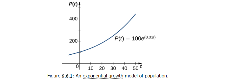
Figure 9.6.19.6.1 shows a graph of P(t)=100e^0.03t
P0=100
R=0.03.
We can verify that the function.
P(t)=P0e^rt satisfying the initial values dp/dt=rt
There is a fascinating interpretation for this differential equation. The pace at which the population grows (or shrinks) is shown on the left-hand side. The right-hand side is equal to the current population times a positive constant. Therefore, according to the differential equation, the rate of population growth is proportionate to the population at that particular period. It also claims that the proportionality constant is a constant.
This function’s assumption that the population would continue to rise unchecked throughout time is one of its flaws. Real-world conditions would not support this. The birth rate, mortality rate, availability of food, presence of predators, and other factors all affect how quickly a population grows. The growth constant r may be thought of as a net (birth minus death) percent growth rate per unit time. It typically only takes into account the birth and death rates, however, and does not account for any other factors. Whether the pace of population expansion is constant throughout time or subject to variation is a logical topic to pose. Researchers in biology have discovered that populations expand until they achieve a certain steady-state population in many biological systems. In the case of exponential growth, this option is not considered. Nevertheless, the idea of carrying capacity allows for the potential that only a specific number of a given creature or animal may flourish in a given location without encountering resource problems.
Let K be a specific organism’s environmental carrying capacity, and let r denote the growth rate as a real integer. The starting population (the population of the organism at time t=0) is represented by the constant P0, and the population of this organism as a function of time t is represented by the function P(t). The logistic differential equation is then.
dP/dt =rP(1−P/K).
Pierre Verhulst initially published the logistic equation in 1845. An initial-value issue for P(t) may be created using this differential equation and the initial condition P(0)=P0.
Consider a situation where the beginning population is low in comparison to the carrying capacity. If so, P/K is low and may even be close to zero. As a result, the amount included in parentheses on Equation above right side is near to 1 and the right side of this equation is close to rP. If r>0, the population expands quickly in a manner akin to exponential growth.
But because K is constant, as the population expands, so does the ratio P/K. P/K is smaller than 1, therefore 1P/K>0, if the population stays below the carrying limit. As a result, the Equation above right-hand side is still positive, but the amount in parentheses lowers and the growth rate declines as a result. The population stays the same if P=K since the right-hand side is equal to zero. Let’s say that the population is larger in the beginning than the carrying capacity. Then P/K>1 and 1P/K<0 follow. The population declines when the right side of the Equation is negative. Population declines as long as P>K. The population approaches the carrying capacity as t approaches infinity, but it never fully hits K since dP/dt will continue to shrink. A phase line is a visual representation of this analysis. Depending on the original situation, a phase line defines the general behavior of a solution to an autonomous differential equation.

© 2024 MAT 2680 Differential Equations Spring 2023
Theme by Anders Noren — Up ↑
The OpenLab is an open-source, digital platform designed to support teaching and learning at City Tech (New York City College of Technology), and to promote student and faculty engagement in the intellectual and social life of the college community.


Recent Comments