Category: Tutorials (Page 1 of 2)

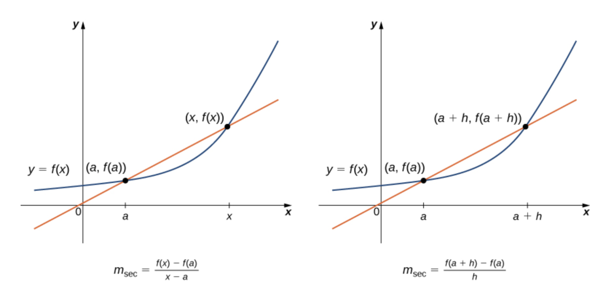
The Chain Rule is the following (taken from Sec 3.6 of the textbook)–it shows how to compute the derivative of a composite function h(x) = f(g(x)):

The key to using the Chain Rule is to analyze a given composite function in terms of the “outside function” (the function f in the notation above) and the “inside function” (g above). The Chain Rule says the derivative of the composite function is “the derivative of the outside function evaluated at the inside function” (i.e., f'(g(x))) times “the derivative of the inside function” (i.e., g'(x)).

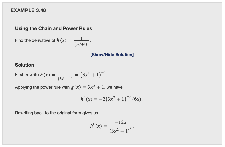
Here are a couple examples from the textbook. In Example 3.49, for h(x) = (sin x)^3, the “outside function” is the cubing function f(u) = u^3, and the “inside function” is g(x) = sin x:

What are the “outside” and “inside” functions in the following example?

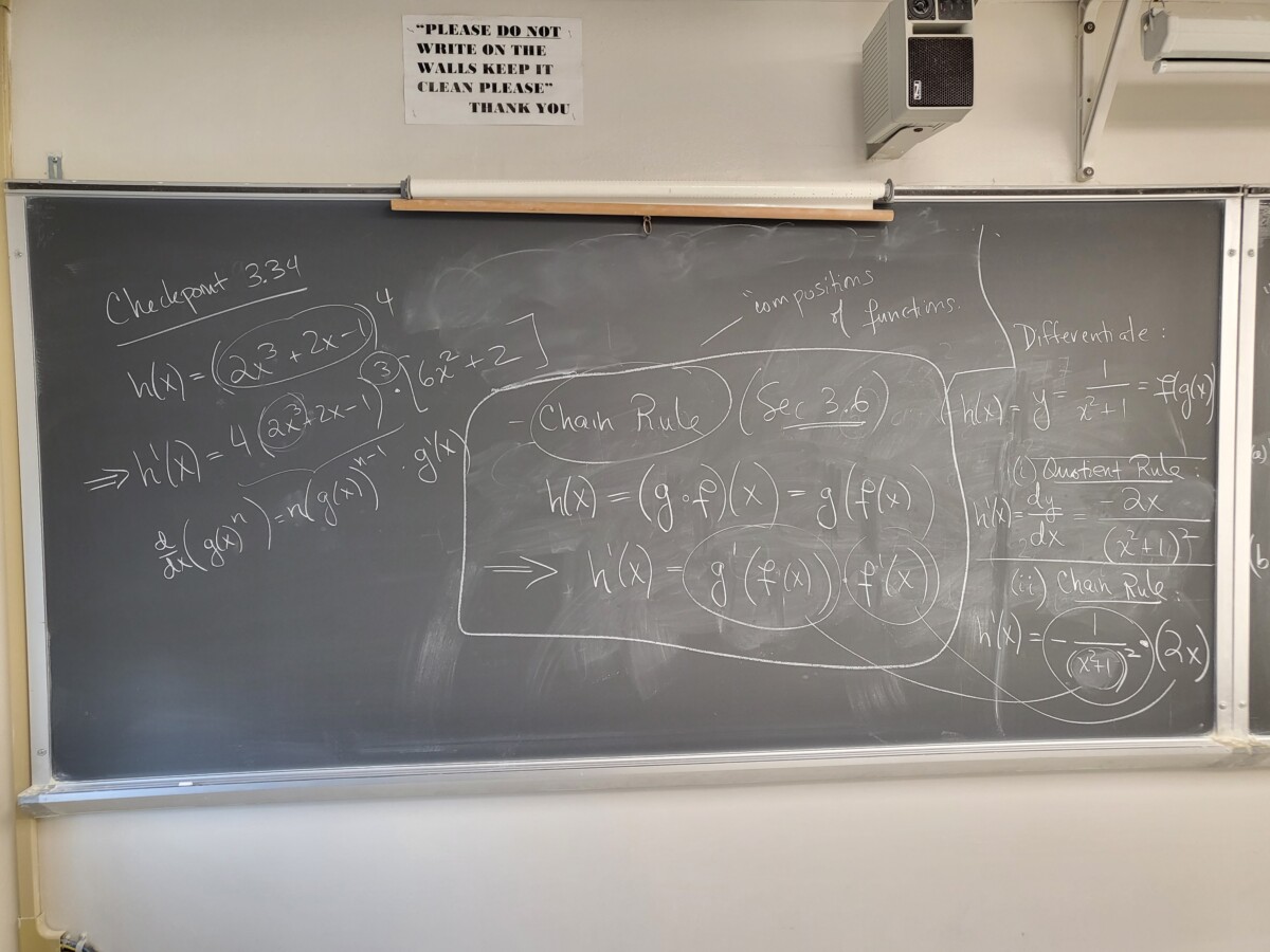
Here is the Chain Rule as I presented it in class (but note that I wrote it out there applied to h(x) = g(f(x))), along with another “Checkpoint” example from the textbook:

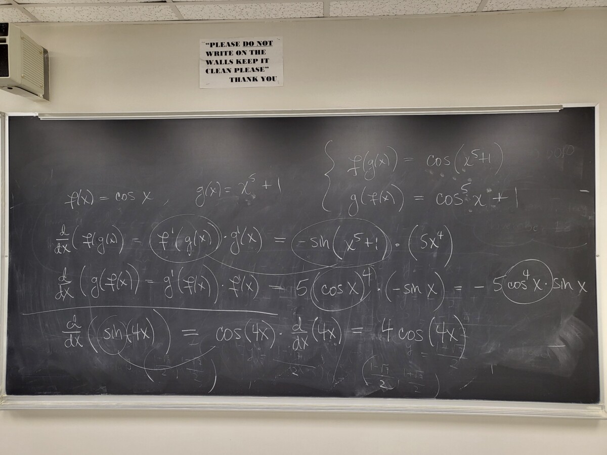
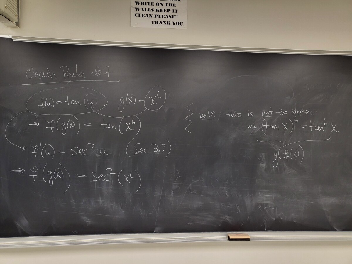
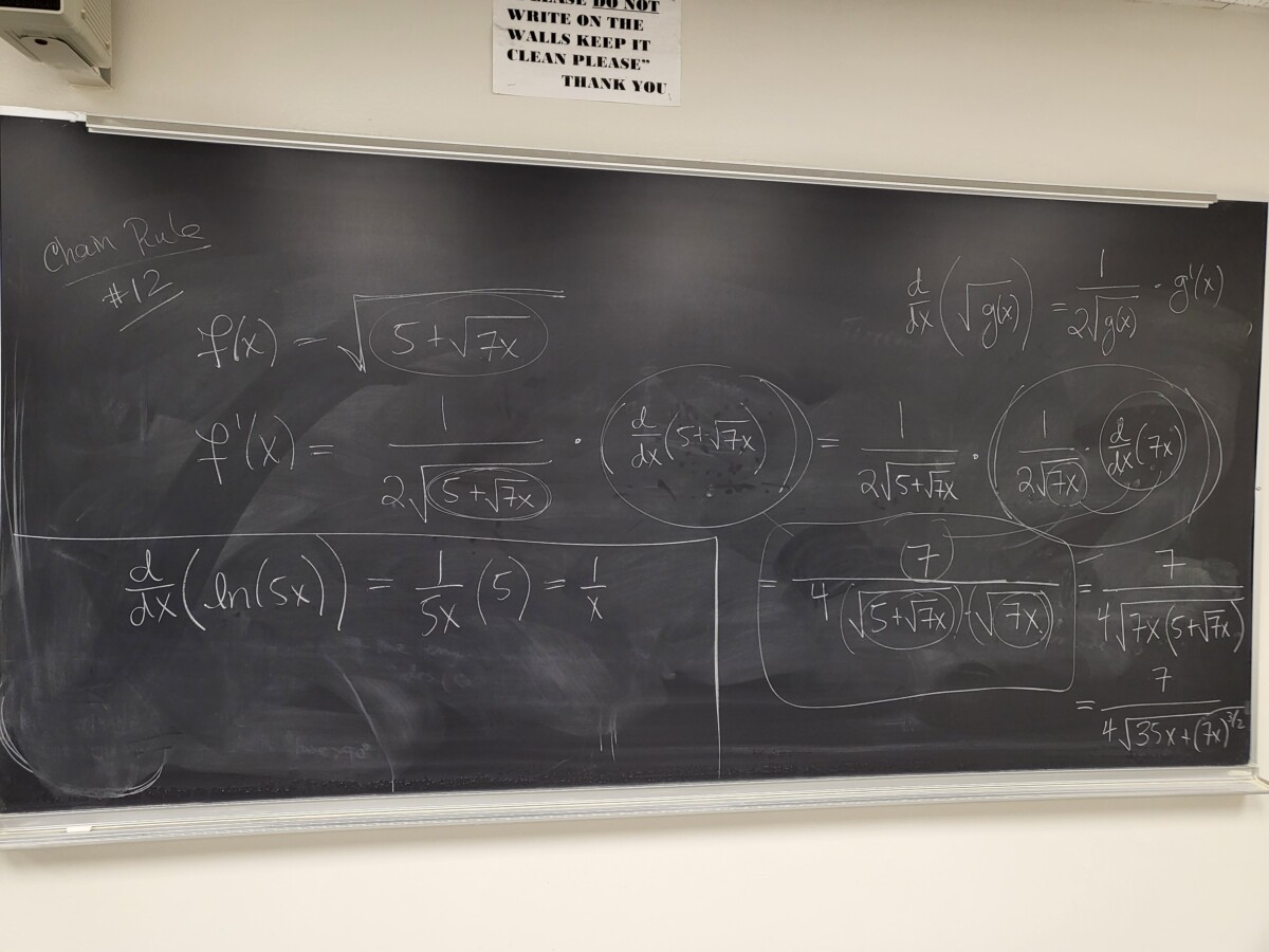
Here are a few more Chain Rule examples we did in class:

As we’ve been saying all semester, the key idea of “differential calculus” (i.e., this course) is the definition of the derivative, and how it captures “the instantaneous rate of change” (which is the same as the slope of the tangent line) as the limit of average rates of change (the limit of slopes of secant lines).

Here is the key figure again:

Note that “m_sec” is the slope of the secant line passing through the points (a, f(a)) and (x, f(x)). But this ratio (the difference quotient) is also the average rate of change of f over the x-interval (a, x)!

Here is the same figure again, as I sketched on the board last week:

Here is this concept applied to Problem 1 of “Derivatives – Rates of Change”:

Where do we get these solutions? From the following calculations:

Since the derivative of a function gives us it’s instantaneous rate of change, the derivative of a “position function” s(t) gives us velocity. And the derivative of velocity, i.e., the rate of change of velocity, is gives us acceleration. Here is an excerpt from the textbook:

Here is an exercise from the WebWork set:

We get the velocity function v(t) by differentiating the given s(t), i.e., v(t) = s'(t); and we get the acceleration function a(t) by differentiating v(t), i.e., a(t) = v'(t) = s”(t).

In order to answer (b), note that the particle is “moving in the positive direction” whenever v(t) > 0. We can solve this algebraically or graphically:

Since v(t) = 3t^2 – 4t +1 = (3t – 1)(t – 1), clearly v(t) = 0 for t = 1/3 and t = 1. Since the graph of y = v(t) is a parabola opening upwards, this means v(t) > 0 for t < 1/3 and t > 1, i.e., on (-inf, 1/3) U (1, inf).

But since we are only considering t >= 0, i.e., that is the domain of s(t), as noted at the start of the exercise (t = 0 is when “time starts” for the motion of this particle), the solution is: [0, 1/3) U (1, inf).

Conversely, the solution for (c) consists of the values of t for which v(t) > 0, which is (1/3, 1).

The Product Rule, which we covered in class on Tuesday (Oct 18), is the following (from Sec 3.3 of the textbook)–it shows how to compute the derivative of the product f*g (i.e., f(x)*g(x)):

We covered the following example from the textbook, which is very similar to a couple of the WebWork exercises:

See also the following example:

The Quotient Rule (covered in class on Thurs Oct 20) is the following–it shows how to compute the derivative of the quotient function f/g (i.e., f(x)/g(x)):

It may be helpful to think of the quotient rule in terms of the “top” (numerator) function and “bottom” (denominator) function. Here is how I wrote the quotient rule in class today:

Finally, here is an example from the textbook (in this example, the “top” function is 5x^2 and the “bottom” function is 4x+3):