Lesson 21: Approximating Areas

Motivating question

Why do definite integrals determine areas?

Introduction to Riemann sums – motivating example

Recall from Lesson 2 (link here) that our definition of a definite integral was a signed area. This differed from the textbook’s definition, which we will see later in this lesson. First, let’s look at an example.

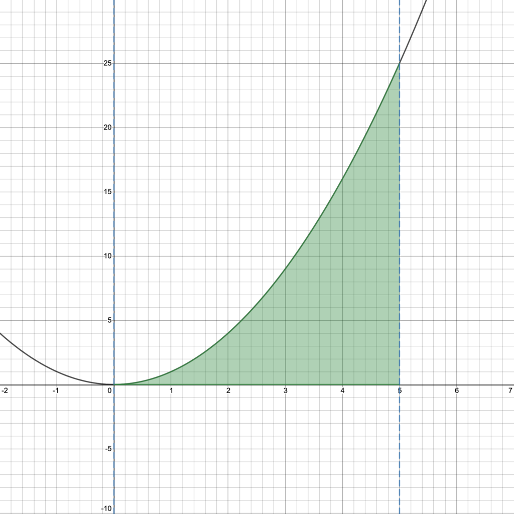
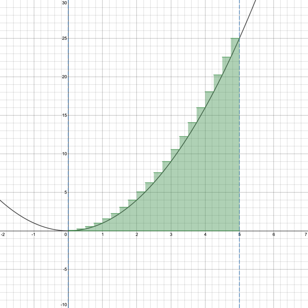
Question: If you didn’t know the Fundamental Theorem of Calculus, how would you evaluate $\int_0^5 x^2 dx$? Figure 1 below shows the irregular shape whose area you are asked to calculate (shaded in green).

There are lots of different ways to answer this question! We are interested in one in particular.

Answer an easier question first

Analogy: Recall from your Calculus I class that when you were first asked to determine the slope of the line tangent to the graph of a function at a point, you couldn’t do it because the slope formula requires two distinct points. But you answer an easier question: you could approximate the slope of the tangent line by choosing a second point on the curve and calculating the slope of the secant line through those two points. And then you could get a better approximation by dragging that second point closer to the first point and calculating the slope of the secant line through those two points. then you could get the actual slope of the tangent by taking a limit of slopes of secants. See an interactive Desmos graph showing the tangent as a limit of secants here; see the corresponding lesson on the MAT 1475 course hub here.

So to begin to answer the question: how can we determine the area of the region represented by $\int_0^5 x^2 dx$, let’s answer an easier question first. In the Calculus I analogy, the easier question was “What is the slope of a secant line that approximates the tangent line?” Here, we’re not trying to determine slope, we’re trying to determine area, so we need to determine a shape whose area is easy for us to calculate and which approximates the area of the shape whose area we’re interested in.

What’s a shape with an easy area? A rectangle! As usual, the area of a rectangle is

\[A = \ell\cdot w\]

where $\ell$ is its length and $w$ is its width.

For our example of $\int_0^5 x^2 dx$, let’s first choose a rectangle whose base (or width) is equal to the base of our irregular shape and whose height (or length) is equal to the height of our irregular shape as in Figure 2.

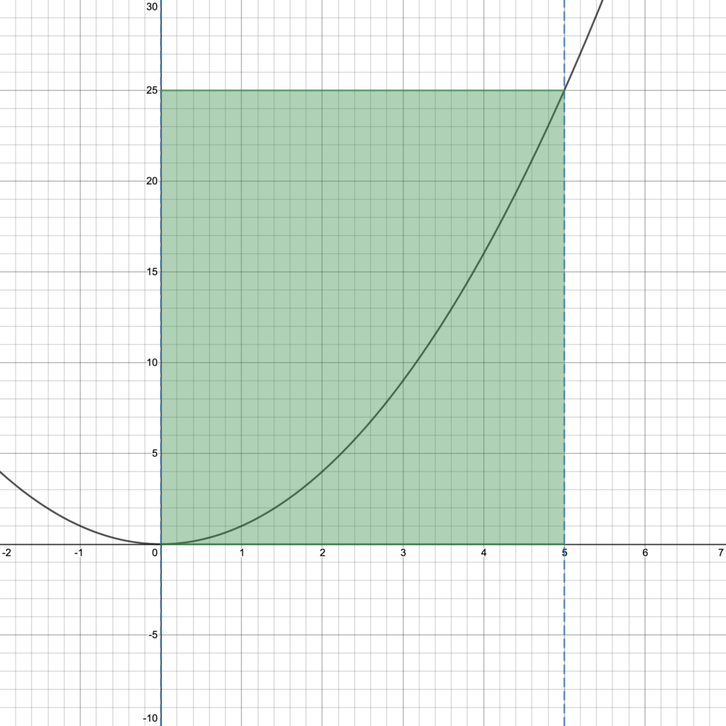
The area of this rectangle is pretty easy to calculate! Its base is the length of the interval [0,5], which is 5-0=5 units. Its height is just the value of the function at the right side of the interval [0,5], which is $f(5) = 5^2 = 25$ units. So the area of this rectangle is $f(5)\cdot 5 = 25 \cdot 5 = 125$ square units.

We can see in Figure 2 that this is not a great approximation, but at least it was easy to find! So how can we do better? How can we use areas of rectangles to find a better approximation? Figure 3 gives us a hint.

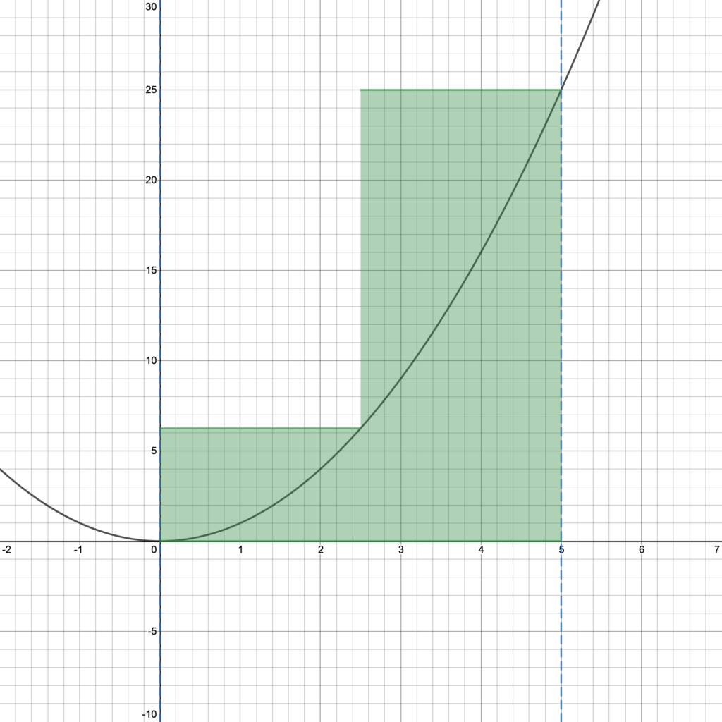
According to Figure 3, by splitting (or “partitioning”) the interval [0,5] into two subintervals [0,2.5] and [2.5,5], we can approximate the area represented by $\int_0^5 x^2 dx$ by the sums of the areas of these two rectangles. Notice that this is a better approximation than the one in Figure 2. The two subintervals have equal length, so they each have length $\frac{5-0}{2} = 2.5$. Since the heights of these rectangles are given by the value of the function at the right endpoints of the subintervals, the sum of the areas of the two rectangles in square units is:

\[f(2.5)\cdot 2.5 + f(5)\cdot 2.5 = (2.5)^2 \cdot 2.5 + 5^2 \cdot 2.5 = 78.125\]

Now maybe you are starting to see the pattern. Rectangles have areas that are easy to calculate! The more rectangles the better the approximation! Figure 4 shows an approximation with 20 rectangles; click on Figure 4 to see an interactive Desmos graph where you can change

• $n$, the number of rectangles,
• $a$, the left interval endpoint (lower limit of integration),
• $b$, the right interval endpoint (upper limit of integration),
• $f(x)$, the function whose graph gives the upper boundary of the region.

Another example

In most cases, we will be interested in examples where each of the rectangles have the same base (width). Video 1 shows another example where the rectangles used don’t necessarily have the same base because the subintervals are of different lengths.

Main idea, notation, and formula

The main idea of Riemann sums is that you can approximate the area of a region by chopping it into bits and then adding up the approximate areas of each bit. The more bits you have, the smaller they are, and the better the approximation. Integration is just the limit of this: you are adding up the areas of infinitely many infinitely small bits.

First we want a formula for an approximate the area represented by $\int_a^b f(x)dx$. To write this formula, we need some notation. We will make some assumptions:

• there are $n$ subintervals of $[a,b]$ (so there are $n$ rectangles),
• each subinterval has the same length, which will be $\frac{b-a}{n}$; we denote $\frac{b-a}{n}$ by $\Delta x$,
• for $i = 1, 2, \dots, n$, let $x_i^*$ be a point in the $i$th subinterval (we often choose $x_i^*$ to be the left endpoint or right endpoint in the subinterval—our examples above all used the right endpoint),
• the height of the $i$th rectangle is given by $f(x_i^*)$.

With this notation, the $i$th rectangle has area $f(x_i^*) \Delta x$ and the approximation of $\int_a^b f(x)dx$ by $n$ rectangles is given by

\[ \int_a^b f(x)dx \approx \sum_{i=1}^n f(x_i^*) \Delta x.\]

This is called a Riemann sum. Notice that as the number $n$ of rectangles increases, the skinnier they get. This means that as $n$ increases, $\Delta x$ decreases. In the limit, as $n$ approaches $\infty$, $\Delta x$ approaches 0 and the rectangles become infinitely thin strips. As the number $n$ of rectangles increases, the better the approximation.

Now we’re ready for a formula that gives us the actual area. Compare this with the definition in our text here. Remember the Calculus I analogy above: the slope of the tangent line is the limit of the slopes of the secant lines. Here, we see that the area under the curve is the limit of the sum of areas of rectangles.

It’s helpful to see the similarities between the expression on the left and the expression on the right.

1. First let’s look at the symbols $\int$ and $\sum$:
   • on the right the letter $\sum$ “sigma” is the capital Greek letter S, which stands for sum,
   • on the left we have $\int$ which is like an elongated letter S; $\int$ represents an infinite sum of infinitely small terms.
2. Now let’s look at the symbols $dx$ and $\Delta x$:
   • on the right we have $\Delta x$ where $\Delta$ “delta” is the capital Greek letter D, which stands for difference,
   • on the left we have $dx$, which represents an infinitely small difference; recall the analogy with slopes in Calculus 1: $\lim_{\Delta x \to \infty} \frac{\Delta y}{\Delta x} = \frac{dy}{dx}.$
3. Finally, we notice that $f(x)$ appears in the integrand on the left and $f(x_i^*)$ appears in the finite sum on the right.

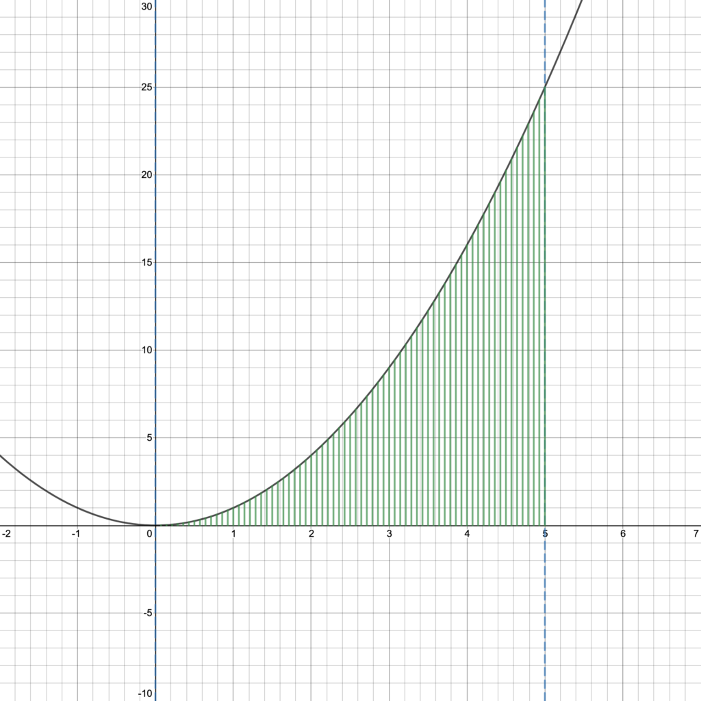
With these similarities in mind, we can think about $\int_a^b f(x) dx$ as representing an “infinite sum of heights”—areas of rectangles, each of which is infinitely thin. While this is not entirely precise, it helps us understand what is happening in the limit as $n$ approaches $\infty$. In some sense, by integrating $f(x)$ between $x=a$ and $x=b$, we are adding up a whole 1-dimensional family of 1-dimensional heights to get a 2-dimensional area. Figure 4 shows this idea with a family of only 70 heights between $a=0$ and $b=5$. This picture of integrating heights to find area will help us again in upcoming lessons on using integrals to find volume of 3-dimensional shapes.

More examples

Videos 2, 3, and 4 shows an example where the subintervals all have the same length and where $x_i^*$ is the left endpoint, right endpoint, and midpoint of the $i$th subinterval respectively.

Videos 5 and 6 show two more examples where the subintervals have different lengths.

Your textbook uses notation $L_n$ to represent the Riemann sum with $n$ rectangles where $x_i^*$ is the left endpoint of the $i$th subinterval and $R_n$ to represent the Riemann sum with $n$ rectangles where $x_i^*$ is the right endpoint of the $i$th subinterval.