Welcome back! For the next few lessons, it might look like we’re changing topics completely, but recall the questions at the end of the lessons on Taylor polynomials (link to Lesson 11 here and link to Lesson 12 here). Over the next several sessions we’ll work on making those questions more precise and then we’ll work on answering them in Lessons 19 and 20.

Lesson 13: Sequences
Learning goals:
- Find the formula for the general term of a sequence.
- Calculate the limit of a sequence if it exists.
- Determine the convergence or divergence of a given sequence.
Motivating question
At the end of Lessons 11 and 12 we asked questions about which Taylor polynomial would “best approximate” a function. The question isn’t quite precise yet, but we can guess that the answer should be something like an “infinite-degree polynomial.” Polynomials have finite degrees, though, but we can imagine something like a polynomial that has infinitely many terms which are higher and higher powers of $x$ (with a coefficient). Starting with Lesson 19, we’ll make sense of what it means to “add up infinitely many powers of $x$.” But before we can do that, starting with Lesson 14, we have to make sense of what it means to add up infinitely many numbers. But before we can do that, we have to make sense of what it means to have a list of infinitely many numbers that we want to add up. That’s what our goal is today.
So, what does it mean to have a list of infinitely many numbers?
Evaluate the limit:
\[\lim_{x \to \infty} \frac{1}{x}.\]
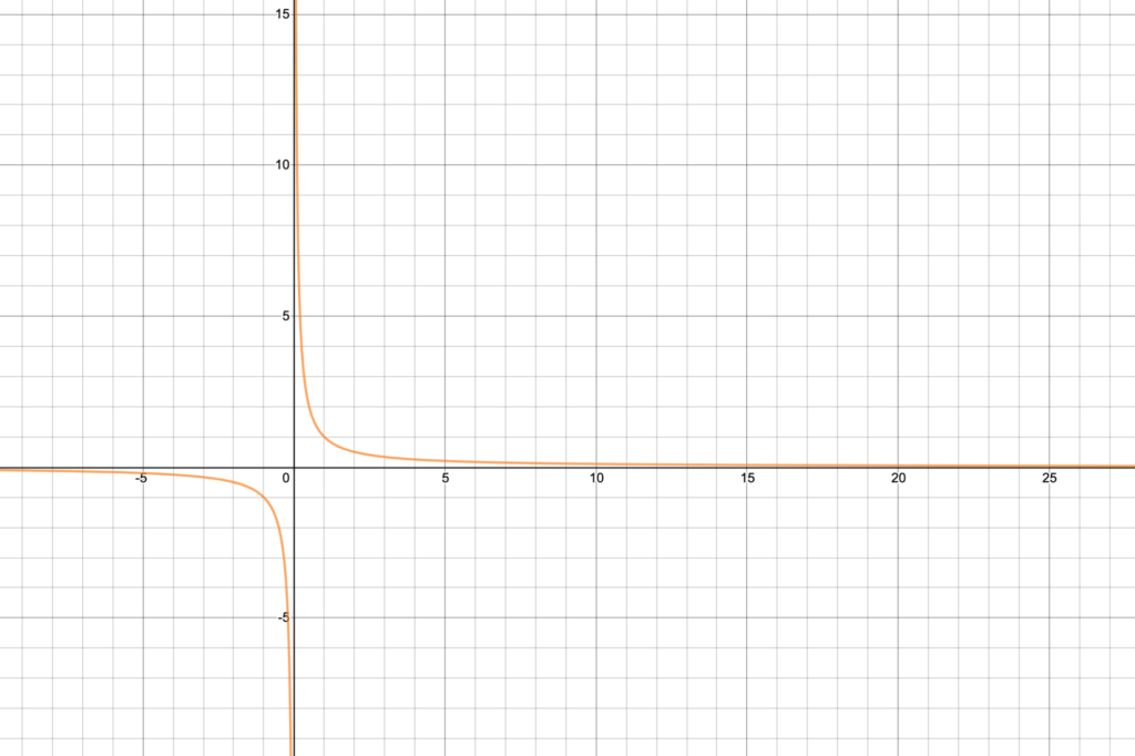
There are different ways for us to say this, but they all amount to approximately the same thing: for any small positive number $\varepsilon$, there is an $x$-value $M$ so that as long as $x > M$, $|f(x)| < \varepsilon$. This just means that $|f(x)|$ gets arbitrarily close to 0 as $x$ gets large. So
\[\lim_{x \to \infty} \frac{1}{x} = 0.\]
Remember that graphically this means that $y=f(x)$ has the $x$-axis as a horizontal asymptote when $x$ approaches $\infty$ as in Figure 1 below.
Evaluate the limit:
\[\lim_{x \to \infty} \left(\frac{1}{2}\right)^x.\]
Again, we can see as $x$ values get large, $f(x)$ gets closer and closer to zero. Again, graphically, this means the graph $y=(\left\frac{1}{2}\right)^x$ has a horizontal asymptote when $x$ approaches $\infty$ as in Figure 2 below.

The landscape: where are we and where are we going?
Recall that eventually we want to make sense of something like:
\[x + \frac{1}{2}x^2+ \frac{1}{3}x^3+ \frac{1}{4}x^4+ \frac{1}{5}x^5+ \frac{1}{6}x^6+\dots \]
(where $\dots$ means the sum goes on forever following the same pattern). First we’ll make sense of something like:
\[1 + \frac{1}{2}+ \frac{1}{3}+ \frac{1}{4}+ \frac{1}{5}+ \frac{1}{6}+ \dots.\]
But first we’ll need to make sense of something like:
\[1, \frac{1}{2}, \frac{1}{3}, \frac{1}{4}, \frac{1}{5}, \frac{1}{6}, \dots.\]
This is our first example of a sequence.
Sequences
Definition:
- A finite sequence is a finite ordered list of numbers $a_1, a_2, a_3, \dots, a_n$.
- An infinite sequence is an infinite ordered list of numbers $a_1, a_2, a_3, \dots$.
Notice that the list is ordered, but the numbers themselves don’t have to be in order. So, for example, $1, 8, 20, -5, \frac{1}{10}, 0.5, \sqrt{2}, \pi$ is a perfectly good sequence. This sequence is finite since the list ends. The first number in the sequence is $1$ so $a_1 = 1$; the second number is $8$ so $a_2 = 8$; the third number is $20$ so $a_3=20$; and so on.
Some sequences follow a pattern. In the example above $1, \frac{1}{2}, \frac{1}{3}, \frac{1}{4}, \frac{1}{5}, \frac{1}{6}, \dots$, we can determine a formula for the general term $a_n$. Since $a_1 = 1$, $a_2 = \frac{1}{2}$, $a_3 = \frac{1}{3}$, and so on, we can see that we can write the general term as a formula in terms of $n$: $a_n = \frac{1}{n}$.
Just a function
The last example in particular demonstrates that a sequence is just a function whose domain is the natural numbers $1, 2, 3, \dots$. It might help to use the notation $f(n) = a_n$. So in our example above, $a_n = \frac{1}{n}$ is the same thing as the function $f(x) = \frac{1}{x}$, but with the domain restricted to the natural numbers. We can even graph the sequence just as we graph the function. Figure 3 below shows the function $f(x) = \frac{1}{x}$ (without restricting the domain) and the sequence $a_n = \frac{1}{n}$ graphed together. The orange curve is the graph of $f(x)$ and the blue points represent the sequence $a_n$. Notice that the coordinates of the points are of the form $(n, a_n)$ where $n$ is a natural number.

Closed form of a sequence
In the previous example, we call the formula for the general term $a_n$ in terms of $n$ the closed form of the sequence. This is particularly nice because we can do just one calculation to get any term in the sequence. For example, we know that $a_{100} = \frac{1}{100}$.
Recursively defined sequences
Other sequences might follow a pattern, but it might not be given as a closed form. Example. you may have seen the following sequence:
\[1, 1, 2, 3, 5, 8, 13, 21, \dots.\]
This is known as the Fibonacci sequence and it appears all over in mathematics and nature. Can you see the pattern?
Determine the formula for the general term $a_n$ of the Fibonacci sequence $1, 1, 2, 3, 5, 8, 13, 21, \dots$.
Hint: give yourself a few minutes to play around with this before checking the answer below, especially if you haven’t seen it before.
Once we have the first two terms of the sequence, we can build the rest by taking the sum of the previous two terms.
- $a_1 = 1$
- $a_2 = 1$
- $a_3 = a_1+a_2 = 1+1=2$
- $a_4 = a_2+a_3=1+2=3$
- $a_5=a_3+a_4 = 2+3=5$
- $a_6 = a_4+a_5 = 3+5=8$
- and so on…
We’d like to have a formula for the general term $a_n$. The term that comes before $a_n$ is $a_{n-1}$ and the term that comes before $a_{n-1}$ is $a_{n-2}$. Since any term is the sum of the previous two terms, $a_n = a_{n-2}+a_{n-1}$. For the complete definition, we need to include what the first two terms are, since they can’t be determined using this formula. So the complete definition is:
\[a_1=1, a_2=1, a_n=a_{n-2}+a_{n-1} \;{\rm for } \;n > 2.\]
We say that sequences like the Fibonacci sequence are recursively defined. This means that the general term $a_n$ of the sequence is given in terms of previous terms of the sequence, not in terms of $n$ itself. Recursive definitions are not usually as nice as closed forms, because you can’t calculate a specific term directly. For example, if we wanted to know the hundredth term $a_{100}$…well…$a_{100} = a_{98}+a_{99}$, so we’d have to calculate $a_{99}$ and $a_{98}$. But $a_{99} = a_{97}+a_{98}$, so we’d have to calculate $a_{97}$ too. You can see, that actually this would be a lot of calculations! Compare this to the example where $a_n =\frac{1}{n}$ so $a_{100} = \frac{1}{100}$. We were able to say what the hundredth term was with one easy calculation because we had a closed form for $a_n$.
Some recursive sequences do in fact have a closed form as well as a recursive definition. You may have seen how to find the closed form of the Fibonacci sequence in your Discrete Math or Algorithms class; it takes some work to find it and is outside the scope of this class.
Geometric sequences
You may have seen arithmetic and geometric sequences in your precalculus class. These are two other special types of sequences. For our purposes, the geometric sequences will be more relevant so we will ignore arithmetic sequences for the most part.
Definition: A geometric sequence is one of the form $a, ar, ar^2, ar^3, ar^4, \dots$. Its closed form is
\[a_n = ar^{n-1}.\]
Geometric sequences (and geometric series, which we’ll study later) are extremely nice, because if you know the first term $a$ and you know the common ratio $r$, then you know the whole sequence.
Example. One geometric sequence that we’ll come back to is given by $a_n = \left( \frac{1}{2}\right)^n$. The first few terms are $\frac{1}{2}, \frac{1}{4}, \frac{1}{8}, \frac{1}{16}, \dots$. To see that this is indeed a geometric sequence, we need to determine $a$ and $r$. It will be helpful to write $\left( \frac{1}{2}\right)^n$ as $\frac{1}{2}\left( \frac{1}{2}\right)^{n-1}$. This formula is now of the form $ar^{n-1}$ so we can see that $a$ and $r$ are both $\frac{1}{2}$. Figure 4 below shows the graph of the corresponding function $f(x) = \left( \frac{1}{2}\right)^x$ and the sequence $a_n = \left( \frac{1}{2}\right)^n$.

In general, a geometric sequence $a_n = ar^{n-1}$ corresponds to an exponential function $f(x) = cb^x$ where the domain has been restricted. Everything we know about exponential functions translates nicely to sequences.
Video 1 below takes us through these concepts with some more examples.
Videos 2 and 3 below focuse on geometric sequences.
Convergence of sequences
One of the most important properties of a sequence is whether it converges or diverges. Remember from Lesson 10 on improper integrals (link here) that “converges” means “small” in some sense and “diverges” means “big” in some sense.
We’re lucky because we can translate everything we know about limits at infinity and horizontal asymptotes of functions to convergence of sequences.
Definition:
- The sequence $a_n$ converges to the value $L$ if \[\lim_{n \to \infty} a_n = L.\]
- The sequence $a_n$ diverges if it does not converge.
Let’s consider the convergence of examples we’ve seen:
- The sequence $a_n = \frac{1}{n}$ converges to 0 because $\lim_{n \to \infty}\frac{1}{n} = 0$ (see Warmup exercise 1).
- The geometric sequence $a_n = (\left\frac{1}{2}\right)^n$ converges to 0 because $\lim_{n \to \infty} (\left\frac{1}{2}\right)^n = 0$ (see Warmup exercise 2).
- The Fibonacci sequence diverges because the limit $\lim_{n \to \infty} a_n$ does not exist. We can see that the terms of the Fibonacci sequence get bigger and bigger, so the limit cannot exist and the sequence must diverge.
Videos 4 and 5 below show some more examples of convergence and divergence of sequences.
Other ways to prove convergence
If a sequence converges, you can sometimes show directly that it converges by showing what value it converges to. If you don’t need to know what value the sequence converges to, if you just want to show that it converges, there are some other tools that you can use.
Monotone convergence theorem
Theorem: If a sequence is bounded and monotonic then it converges.
To understand this theorem, we need to know what it means to be bounded and we need to know what it means to be monotonic. Video 6 below defines these terms for us, helps us understand the statement of the theorem, and shows us how to apply it to a particular example.
Coming up…don’t get it twisted!
Today we discussed the convergence and divergence of sequences. The next several lessons we will focus on the convergence and divergence of series. It will be easy to forget about sequences once we see so much of series but don’t get it twisted! Convergence of series and convergence of sequences are related but they’re different concepts. In fact, we’ll use convergence of sequences to define convergence of series in Lesson 14 (link here).
Additional Video Resources
Determine whether the sequence converges or diverges. If the sequence converges, find its limit.
\[a_n = \frac{2^n+3^n}{4^n}\]

