Lesson 22: Areas Between Two Curves
Learning goals:
- Determine the area of a region between two curves by integrating with respect to the independent or dependent variable.
Topic:
- Volume 2, Section 2.1 Areas Between Two Curves (link to textbook section)
WeBWorK:
- Applications – Area Between Curves
Motivating question
How can we use integrals to find the area between curves in the plane?
Find the area of the grey shaded region in Figure 1 (a square with a circle removed):

The larger shape is a square with side length $5 cm$, so its area is $25 cm^2$. The smaller shape is a circle with diameter $3 cm$ so its radius is $\frac{3}{2}cm$ and its area is $\pi \left( \frac{3}{2} \right)^2 cm^2 = \frac{9 \pi}{4}cm^2$.
The shaded region is the square with the circle removed, so its area is $25 cm^2 – \frac{9 \pi}{4} cm^2 = \frac{100-9\pi}{4} cm^2$ which is about $17.93 cm^2$.
Determine the area of the red shaded region in Figure 2:

We can see that:
- the left boundary of the shaded region is $x=-3$,
- the right boundary is $x=1$,
- the lower boundary is the $y$-axis $x=0$,
- the upper boundary is the graph $y= x^2$.
This means that the red area is represented by the definite integral:
\[ \int_{-3}^1 x^2 dx.\]
We determine the red area by evaluating this integral:
\begin{align} \int_{-3}^1 x^2 dx &= \left. \frac{x^3}{3}\right|_{-3}^1 \\ &= \frac{1^3}{3} – \frac{(-3)^3}{3} \\ &= \frac{1+27}{3}\\ & = \frac{28}{3} {\rm \; square \; units} \end{align}Determine the area of the blue shaded region in Figure 3:

This blue region is similar to the red one in Figure 2. The only difference is that the upper boundary is now the graph $y=-2x+3$. So the blue area is represented by the definite integral
\[ \int_{-3}^1 (-2x+3) dx.\]
We determine the blue area by evaluating this integral:
\begin{align} \int_{-3}^1 (-2x+3) dx &= \left. -2\frac{x^2}{2} +3x\right|_{-3}^1 \\ &= \left. -x^2 +3x\right|_{-3}^1 \\ &= (-1^2 +3(1))-(-(-3)^2 +3(-3))\\ &= 20 {\rm \; square \; units} \end{align}Motivating example
Now we determine the area of the purple shaded region in Figure 4:

We can see that:
- the left boundary of the shaded region is $x=-3$,
- the right boundary is $x=1$,
- the lower boundary is the graph $y= x^2$,
- the upper boundary is the graph $y= -2x+3$.
This means that the red area is represented by the definite integral:
\[ \int_{-3}^1 ((-2x+3)-(x^2)) dx.\]
In particular, the purple region is equal to the blue region minus the red region, so we’ve already done most of the work to find the area of the purple region. We determine the purple area by evaluating this integral:
\begin{align} \int_{-3}^1 (-2x+3-x^2) dx &= \int_{-3}^1 (-2x+3)dx -\int_{-3}^1(x^2) dx \\ &= 20-\frac{28}{3}\\ &= \frac{32}{3} {\rm \; square \; units} \end{align}Notice that to find the upper and lower limits of integration, we had to find the $x$-coordinates of the intersection points of the two graphs, so we had to solve the equation:
\[x^2 = -2x+3\]
The solutions are $x=-3$ and $x= 1$, so the lower limit of integration is $-3$ and the upper limit of integration is $1$.
More examples
Video 1 below explains this idea in general and shows two more examples.
The next few videos show more examples finding area between graphs of two functions. Notice that in some examples, there is only one intersection point, so a vertical boundary is also given.
Riemann sum picture
Notice that in the motivating example, we integrated with respect to the variable $x$. This means that if we were to set up a Riemann sum to approximate the area, as we did in Lesson 21 (link here), our rectangles would be tall and skinny and stacked horizontally next to each other as in Figure 5.
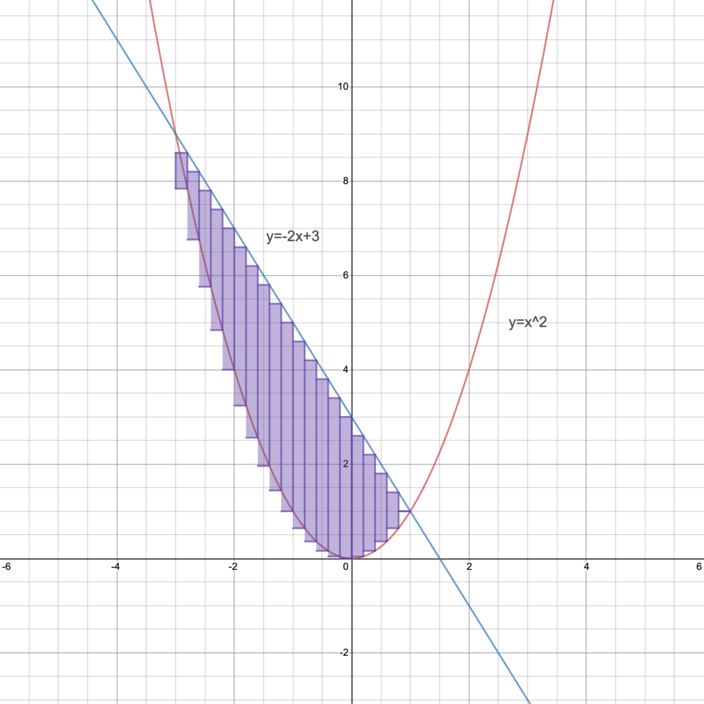
We didn’t have to think about the Riemann sum picture when we were finding the area of the purple shaded region by integrating with respect to $x$; we found the area without Riemann sums! But it’ll help to have this picture in mind for later examples when we are integrating with respect to $y$. We think of this has “horizontal integration,” or “integration with respect to the horizontal coordinate.” So next we’ll perform “vertical integration,” or “integration with respect to the vertical coordinate.” The Riemann sum picture in that case will have thin rectangles on their sides stacked vertically on top of each other.
These pictures of stacking rectangles horizontally or vertically will also come in handy when we are using integrals to compute volumes in Lesson 23 (link here) and Lesson 24 (link here).
Integrating with respect to $y$
In the previous examples where we were finding areas of regions between graphs of functions, our functions gave us $y$ in terms of the variable $x$ and we integrated with respect to $x$. The lower limit of integration was the $x$-coordinate of the left point of intersection (the lowest value of $x$ in the region), and the upper limit of integration was the $x$-coordinate of the right point of intersection (the highest value of $x$ in the region).
When the functions instead give us $x$ in terms of the variable $y$, the procedure is completely analogous. But now we have to integrate with respect to $y$, from the $y$-coordinate of the lower intersection point to the $y$-coordinate of the upper intersection point. Video 6 below shows an example using integration in the vertical direction to find areas of regions between curves.
Additional Video Resources
- Find the area of the region enclosed by the graphs of $y=x^2 – 2x$ and $y = x+4$.
- Find the area of the region enclosed by the graphs of$x=y^2 – 2y$ and $x = y+4$.

