This laboratory experiment main objective is to demonstrate that a three independent loop circuit can be analyze in matlab using mesh analysis by writing a static code in matlab where the components and voltage source can be entered by the user. In this laboratory experiment, complex number will be involve in order to solve for the current and voltages across the three resistors in the circuit. The voltages and current across each resistors will be display in time domain. The program will also display a waveform of the voltage and current across each resistors.

Mesh analysis is a method of analysis use to solve for the current and voltages across elements in a close loop circuit. Mesh analysis is very important technique to solve circuits with many loops. The current flow in each loop can be found by writing mesh equations for each loop and then solving for the current. Mesh equation can be easily solve by using crammers rule. Crammers rule allows to find solution for a system of linear equations with as many equations.

The user will be asked to enter the phase angle of each ac voltage source, for programming purpose the entered angle in degree needs to be converted to radians since matlab makes calculations using radians. Conversion between radians and degree can be easily calculate as follow:

Degrees to radians=(degrees)(PI/180 )

Radians to degree=(radians)(180 /PI)

Since the circuit that will be analyze is an AC-RC circuit, complex numbers are involved when programming to solve the circuit. Matlab allows to find imaginary and real part of complex numbers. The command use to find the imaginary part of a complex number is imag(). The command use to obtain the real part of a complex number is real().

For the purpose of this laboratory experiment, circuit A1 will be analyze.

• First, combine the components to obtain a simpler circuit for coding purposes. As shown in circuit A2.
• Select the loop flow and identify each loop in the circuit.
• Write the linear equation for each loop.
• Write a code in matlab where the user enters the value for each component and voltage source and then the current flow and the voltage drop across each resistor in the circuit is display as well a waveform graph of the current and voltages across each resistor.

Circuit schematics

Circuit A1

Circuit A2

clear
clc
%Input Information
r1= input('Enter value for R1(ohm): ');
r2= input('Enter value for R2(ohm): ');
r3= input('Enter value for R3(ohm): ');
l1= input('Enter value for L1(H): ');
l2= input('Enter value for L2(H): ');
c=input('Enter value for C(F): ');
v1_amp=input('Enter value for V1(V): ');
v1_angle=input('Enter value V1(degree): ');
v2_amp=input('Enter value for V2(V): ');
v2_angle=input('Enter value V2(degree): ');
v3_amp=input('Enter value for V3(V): ');
v3_angle=input('Enter value for(degree): ');
f=input('Enter value for frequency(Hz): ');
%Phasor Domain - rectangular form
w=2*pi*f;
zr1 = r1;
zr2= r2;
zr3=r3;
zl1= +1i*(w*l1);
zl2= +1i*(w*l2);
zc1= -1i*(1/(c*w));
za=zr1+zl1;
zb=zr2+zc1;
zc=zr3+zl2;
v1_rms=v1_amp *.707;
v1_real=v1_rms*cos(v1_angle*(pi/180));
v1_img=v1_rms*sin(v1_angle*(pi/180));
v1=v1_real+v1_img;
v2_rms=v2_amp *.707;
v2_real=v2_rms*cos(v2_angle*(pi/180));
v2_img=v2_rms*sin(v2_angle*(pi/180));
v2=v2_real+v2_img;
v3_rms=v3_amp *.707;
v3_real=v3_rms*cos(v3_angle*(pi/180));
v3_img=v3_rms*sin(v3_angle*(pi/180));
v3=v3_real+v3_img;
%find the matrices for i1,i2,i3
di1=[v1,zb,-za; v2,(zc+zb),zc; v3,zc,(za+zc)];
det_i1=det(di1);
di2=[(za+zb),v1,-za; zb, v2, zc; -za, v3, (za+zc)];
det_i2=det(di2);
di3=[(za+zb),zb,v1; zb,(zb+zc), v2; -za, zc, v3];
det_i3=det(di3);
d=[(za+zb),zb,-za; zb,(zb+zc), zc; -za, zc, (za+zc)];
det_d=det(d);
i1=det_i1/(det_d);
i2=det_i2/(det_d);
i3=det_i3/(det_d);
ir1=i1-i3;
ir2=i2+i1;
ir3=i3+i2;
%display current
time=-1/f:0.01*(1/f):1/f;
ir1_amp=abs(ir1)*sqrt(2);
ir1_angle=angle(ir1)*(180/pi);
ir1t=ir1_amp*sin(w*time + ir1_angle);
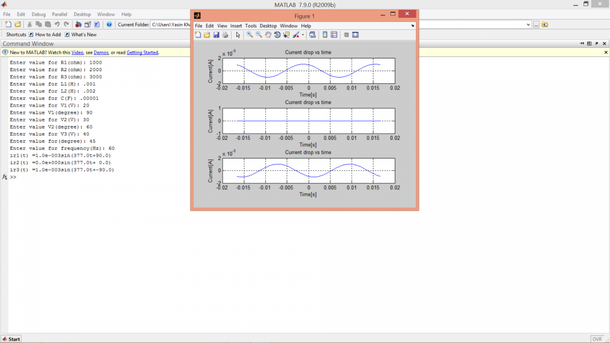
fprintf('ir1(t) =%4.1esin(%4.1ft+%4.1f)\n',ir1_amp,w,ir1_angle);
ir2_amp=abs(ir2)*sqrt(2);
ir2_angle=angle(ir2)*(180/pi);
ir2t=ir2_amp*sin(w*time + ir2_angle);
fprintf('ir2(t) =%4.1esin(%4.1ft+%4.1f)\n',ir2_amp,w,ir2_angle);

ir3_amp=abs(ir3)*sqrt(2);
ir3_angle=angle(ir3)*(180/pi);
ir3t=ir3_amp*sin(w*time + ir3_angle);
fprintf('ir3(t) =%4.1esin(%4.1ft+%4.1f)\n',ir3_amp,w,ir3_angle);
%plot currents

subplot(3,1,1)
%plot ir1,hold all, plot ir2 hold all, plot ir3 hold all
plot(time,ir1t);
title('Current drop vs time')
xlabel('Time[s]')
ylabel ('Current[A]')
grid on
subplot(3,1,2)
plot(time,ir2t);
title('Current drop vs time')
xlabel('Time[s]')
ylabel ('Current[A]')
grid on
subplot(3,1,3)
plot(time,ir3t);
title('Current drop vs time')
xlabel('Time[s]')
ylabel ('Current[A]')
grid on
%plot vr1,hold all, plot vr2 hold all, plot vr3 hold all