Quiz problems:
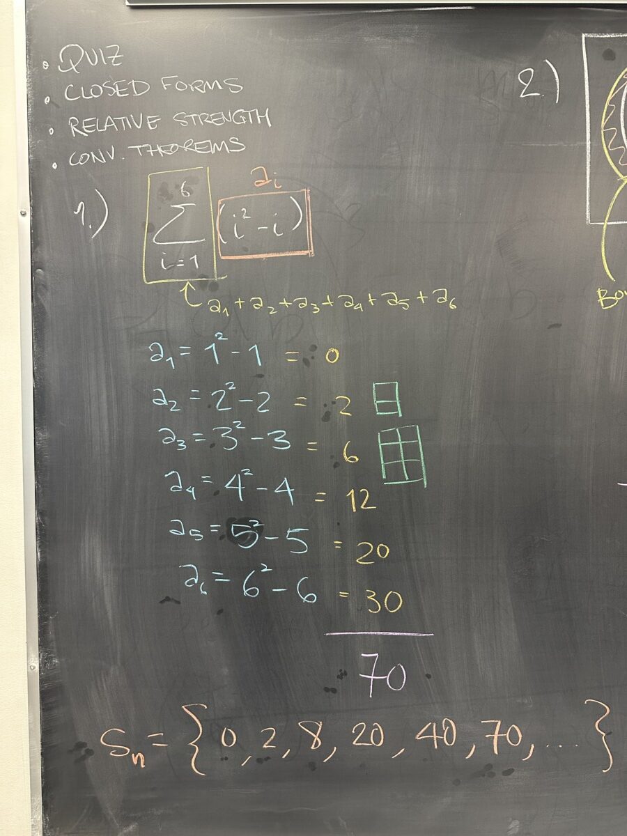
The first quiz problem requested the sixth partial sum for the sequence \( a_i = i^2 – i \). We found the first six terms of the \(a_i\) sequence, then added them up.
Note that this is a recursive approach, as we essentially found all the preceding partial sums in our attempt to find the sixth partial sum.
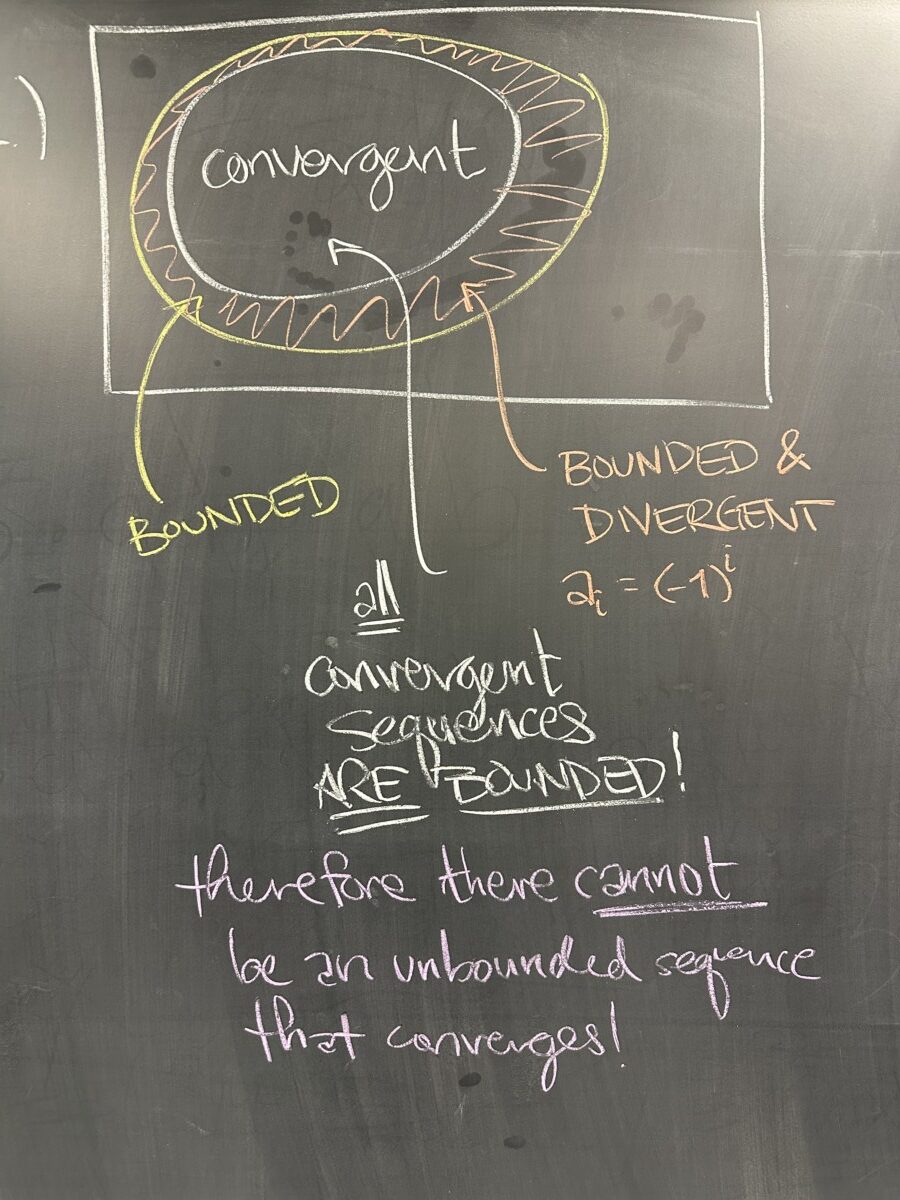
The second quiz question asked about the relationship between a sequence’s “boundedness” and its “convergence”. I used a Venn diagram to explain the relationship between the two properties.
From the diagram it should be (hopefully) clear that all convergent sequences are bounded — AND — some bounded sequences are divergent (such as \(\{1,5,1,5,1,5,\ldots\}\)).
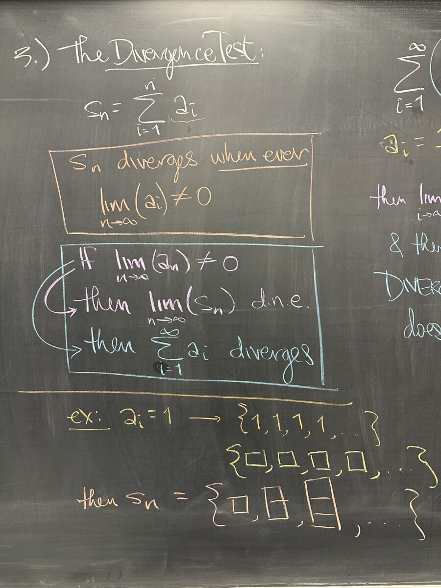
The third quiz question was about the Divergence Test. I stated it several different ways, but the main takeaway is that the Divergence Test ONLY shows divergence.
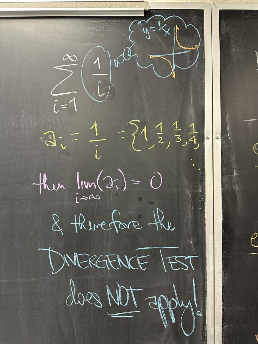
If you have a series such as the one given on the quiz: \(\displaystyle \sum_{i=1}^{\infty} \frac{1}{i}\), with \(\displaystyle\lim_{i\to\infty} a_i = 0\), then Divergence Test does NOT apply.

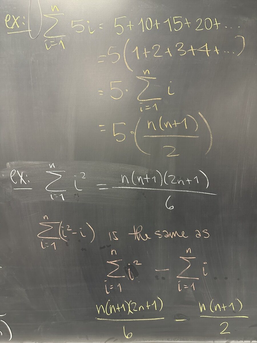
After reviewing the quiz, we got our hands dirty with some “sequences of partial sums” — AKA series.
In each case, we considered the pattern of adding the terms of our \(a_i\) sequence. Once we understood the pattern, we worked out an explicit (closed) formula for the sequence of partial sums.
Knowing the closed form for the sequence of partial sums is useful because the limit of this sequence is the value of our infinite sum.
In each of these six examples, the closed form for \(s_n\) lacks any kind of asymptotic behavior and we should see that the sequences of partial sums are unbounded (and therefore divergent).
Indeed, by looking at each \(a_i\), we can see that the Divergence Test actually applies to each of these examples — further confirming that none of the six examples represent convergent infinite series.

We then turned our attention to comparing the “relative power” of terms which might appear in our sequences. In this picture, we have the fastest growing sequence at the top-right. Every row represents sequences that approach \(\infty\), but the approach is slower each row as we go down. Within each row, the fastest growing sequence is on the right, the slowest on the left.
The final row has no explicit examples, but in-between the unbounded sequences that approach \(\infty\) and the next slide where we look at sequences that approach \(0\), we have sequences that have a finite non-zero limit. An example of this behavior happens when a rational function has the same degree in the numerator and denominator.

On the other side of things, we have sequences that approach zero. As we go down, each row consists of sequences that approach zero faster than the rows above it. Within each row, the sequence that approaches zero fastest is on the right, with slower sequences to the left.
Each of these sequences is a reciprocal of the sequences that approached infinity in the previous slide. More “powerful” sequences that approach infinity also have reciprocals whose values approach zero more quickly.
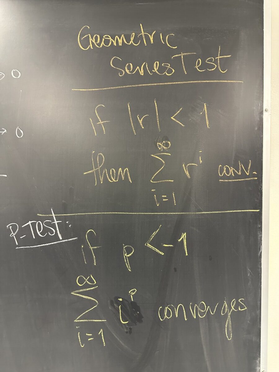
Regarding relative powers, we know we only need to consider series whose sequences have limit zero. Of those, we identify \(a_i = \frac{1}{i}\) (the sequence with power “-1”) as the cutoff between sequences whose series converge and those who diverge. If a sequence has power \(p < -1\) (even \(p=-1.00001\)), its series will converge — i.e. the infinite sum will have a value / the sequence of partial sums will have a limit.
The alternative is also true, if the sequence has power \(p \geq -1\) then its series will diverge.


Recent Comments