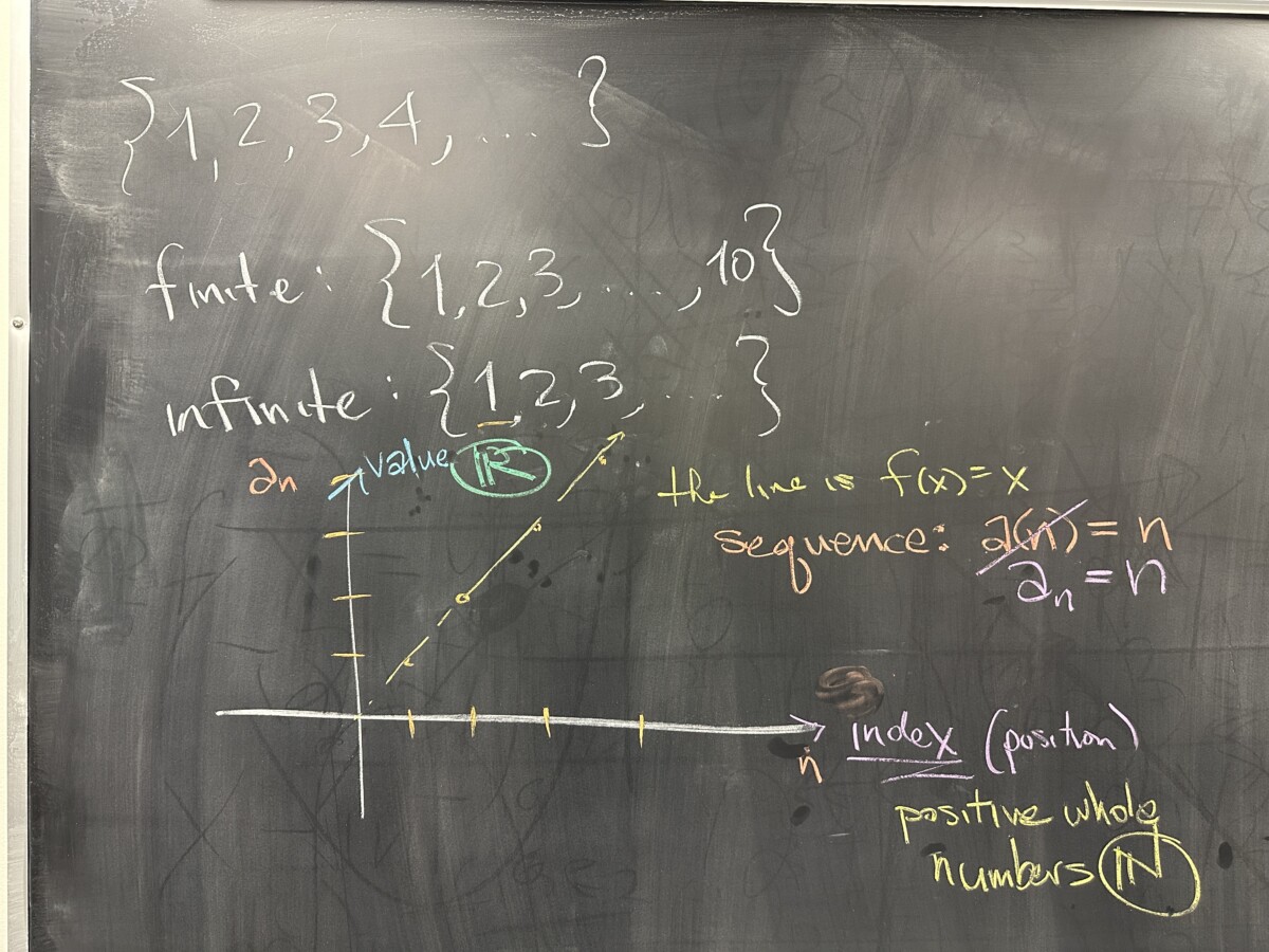
A sequence is an ordered list of values. We can think of the “index” (a.k.a. the position in the sequence) as an input; and we can think of the value located *at* that position as an output. In this way, sequences can also be seen as functions.
The major difference is that sequences only take positive whole numbers as inputs (their domain is \(\mathbb{N}\)).
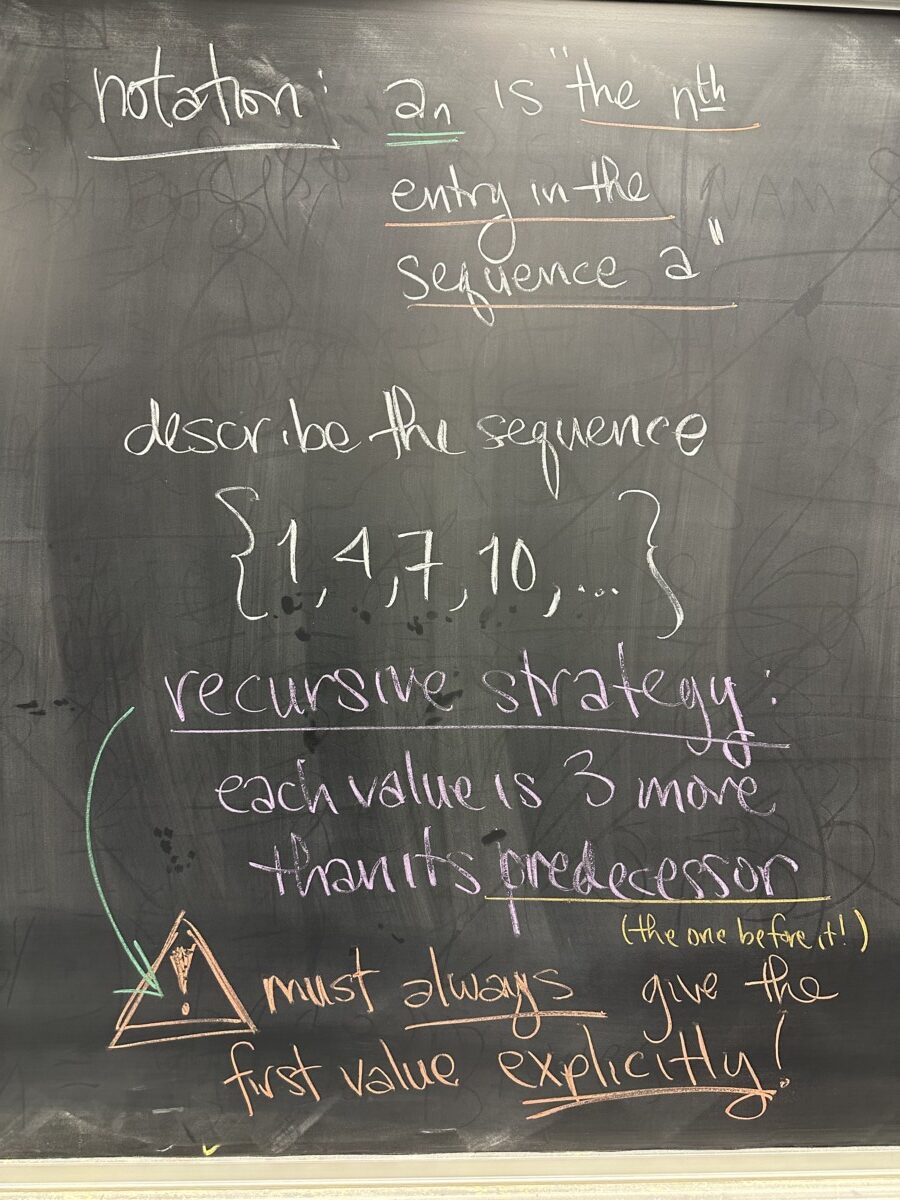
One way to describe the pattern for a sequence is to refer to its previous entries. Such an approach is called “recursion.” Recursion must explicitly state the first value in the sequence because the first value has no previous entries.
In this example, I forgot to write down the algebraic representation in class — so let me do it here: \(a_1 = 1;\text{and}, a_n = 3 + a_{n-1}\)
Literally translated: “the first value is 1” and “each value is 3 more than its predecessor”

The “closed” form of a sequence is a function that depends only on the position whose value we seek.
With recursion, finding \(a_{10}\) would require knowing \(a_9\), which would require knowing \(a_8\), \(a_7\), … and so on. (*Because we can only find a value by adding three to the one before it…)
With the closed form, we will try to skip all that and get right to the value we want.
We noted that we know how many times we must “add three” in order to get from the first value to the tenth value. (nine times)
We noted that in order to find the seventy-second value, we need to “add three” seventy-one times.
In each case, we started with “1” and then “+3” “(n-1)” times.
\(a_n = 1 + 3 \times (n – 1)\)
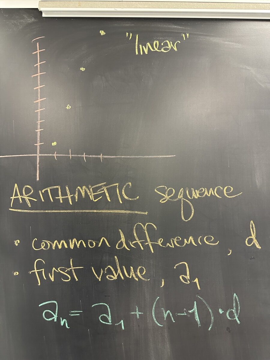
In general, sequences that have this pattern of repeated addition are called “arithmetic” (ahr-ith-MEH-tic rather than ahr-ITH-meh-tic)
They always follow the same general pattern: the first value plus the common difference times (n minus one).
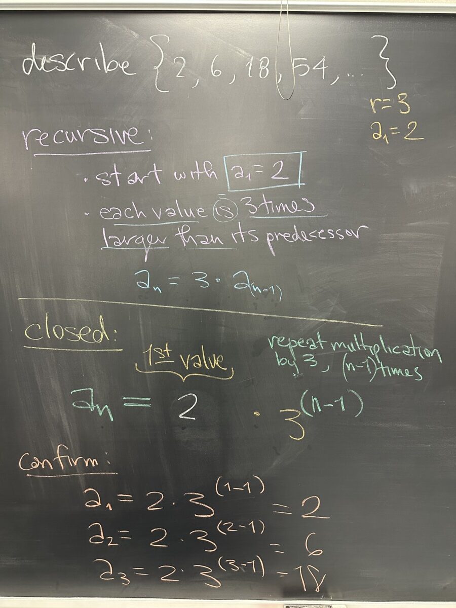
Looking at another example… this time with repeated multiplication rather than repeated addition.
Sequences with this pattern are called “geometric”.
We tackled the recursive description: “start with 2 and then each value is three times its predecessor.” In algebraic notation: \( a_1 = 2; , \text{and} , a_n = 3 \times a_{n-1}\)
We also covered the “closed” description: “two, repeatedly multiplied by three, n minus one times.” In algebraic notation: \(a_n = 2 \times 3^{n-1}\)
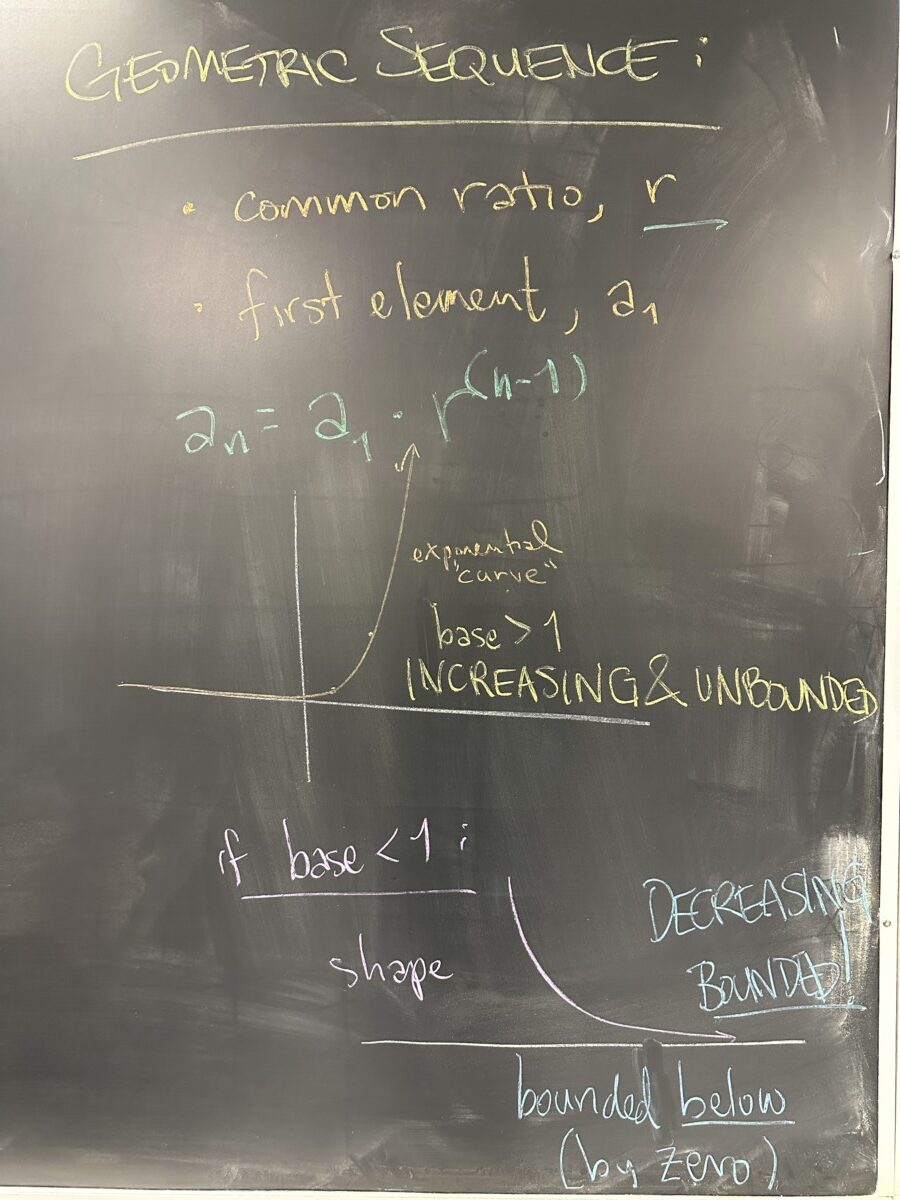
Geometric sequences also have a general form:
\( a_n = a_1 \times r^{n-1} \)
And their general shape follows that of an exponential curve — just as long as the common ratio (the base of our exponential function) is positive!
When a sequence is always “going in the same direction” (e.g. always increasing or always decreasing) it is called monotone. (Often we will specify which direction: “monotone increasing” or “monotone decreasing”.)

We looked at an example where the geometric sequence had a common ratio smaller than 1.
At the very end of class we considered what happens with a geometric sequence that has a negative common ratio. We saw the pattern +,-,+,-,… which we will use the word “alternating” to describe.


Recent Comments