
Before talking about sequences, we started with Zeno’s Paradox (specifically the “dichotomy paradox” — see also the variant “Achilles and the Tortoise”). Under this premise, we considered two values: how many steps we’ve taken (\(n\)) and the distance travelled during that step (\(a_n\)). We think of the term \(a_n\) similar to how we think of \(f(x)\) in that \(f(3)\) means replacing \(x\) with \(3\) just as \(a_3\) means replacing \(n\) with \(3\). Similarly, these values are paired — such as \(n=3\) with \(a_3 = \frac18\) — joining the number of steps with the distance travelled in that step.
We think of \(a_n\) as representing of function of \(n\) just as \(f(x)\) represents a function of \(x\). Note that we use \(n\) as our independent variable instead of \(x\) because we want a variable that only represents whole positive numbers — and \(x\) is already ingrained in us to represent any real number.
Again, as with functions where \(y=f(x)\) is the dependent variable, we write \(a_n\) to represent the dependent variable for sequences. This is also true for specific values: \(x=3,\,y=f(3)\) or \(n=3,\,y=a_3\), we think of these independent/dependent (input/output) values in pairs.

There are two ways to algebraically express the output-values for a sequence, and the first one that the class came up with was “closed form”. This is the most function-like of the two ways. The “closed form” for a sequence is a single algebraic expression that relates the input values, \(n\), to the output values \(a_n\). In our example using Zeno’s Paradox, \(a_n = (\frac12)^n\) is the closed form.
The second way is the “recursive form”. From this perspective, we use algebra to express how to get from one term of the sequence to the next. In other words, we express the output value at the \(n^\text{th}\) step relative to its immediate predecessor, the n-minus-first step. The output at the \(n^\text{th}\) step is \(a_n\) and its predecessor is \(a_{n-1}\). In our example using Zeno’s Paradox, the output at the \(n^\text{th}\) step is half of its predecessor: \(a_n = \frac12 a_{n-1}\).
There is another important piece whenever we use the recursive form, which is discussed later — and that is explicitly stating where the sequence begins (the “initial term”).

There are two important classifications for sequences, the first of which is “monotone”. Saying that a sequence is “monotone” is saying that the output values are always either increasing or decreasing. A sequence such as \(\{4,2,1,2,4,8,\ldots\}\) is not monotone because \(4\rightarrow2\rightarrow1\) is decreasing, but then \(1\rightarrow2\rightarrow4\) is increasing — it’s not strictly one or the other.
When we call a sequence monotone, we always indicate the direction is is taking: either “monotone increasing” or “monotone decreasing”. A monotone increasing sequence satisfies the condition \(a_n > a_{n-1}\) for all \(n\) — in other words, each term of the sequence is larger than its predecessor.
A monotone decreasing sequence satifies the condition \(a_n < a_{n-1}\) for all \(n\) — in other words, each term of the sequence is less than its predecessor.
Then there is the second important classification: whether or not a sequence is “bounded”. A “bounded” function has both an upper and lower bound — values that the sequence never goes beyond.
Using our example from Zeno’s Paradox, we know that our values will never be smaller than zero, nor ever larger than 1. It is important to note that bounded sequences have lots of upper and lower bounds — even in our example, our sequence never gets larger than \(\frac12\), but that means it also never gets larger than \(1\), or larger than \(10\), or \(100\), or … you get the point, I hope, bounds don’t have to be specific values.

But the most important classification for sequences is that of “convergence” or “divergence”. If a sequence has “asymptotic behavior” (as in stabilizing towards some fixed output value), we say the sequence “converges” or “is convergent”.
Saying that a sequence converges is equivalent to saying that it “has a limit”. Moreover, we usually specify the value to which the sequence converges — as we similarly do for limits, we usually give the value of the limit (rather than simply saying that the limit exists). In the case of Zeno’s Paradox, we see asymptotic behavior (\(a_n=(\frac12)^n\) behaves similarly to \(f(x)=(\frac12)^n\)) as the terms continue to shrink by a factor of \(\frac12\) towards zero. In other words, \(\displaystyle\lim_{n\to\infty}\left(\frac12\right)^n=0\). In conclusion, we say that \(a_n\) converges to \(0\).
Although our initial example was both bounded and monotone, we have plenty of other examples to look at that are only one or the other — or even perhaps neither.
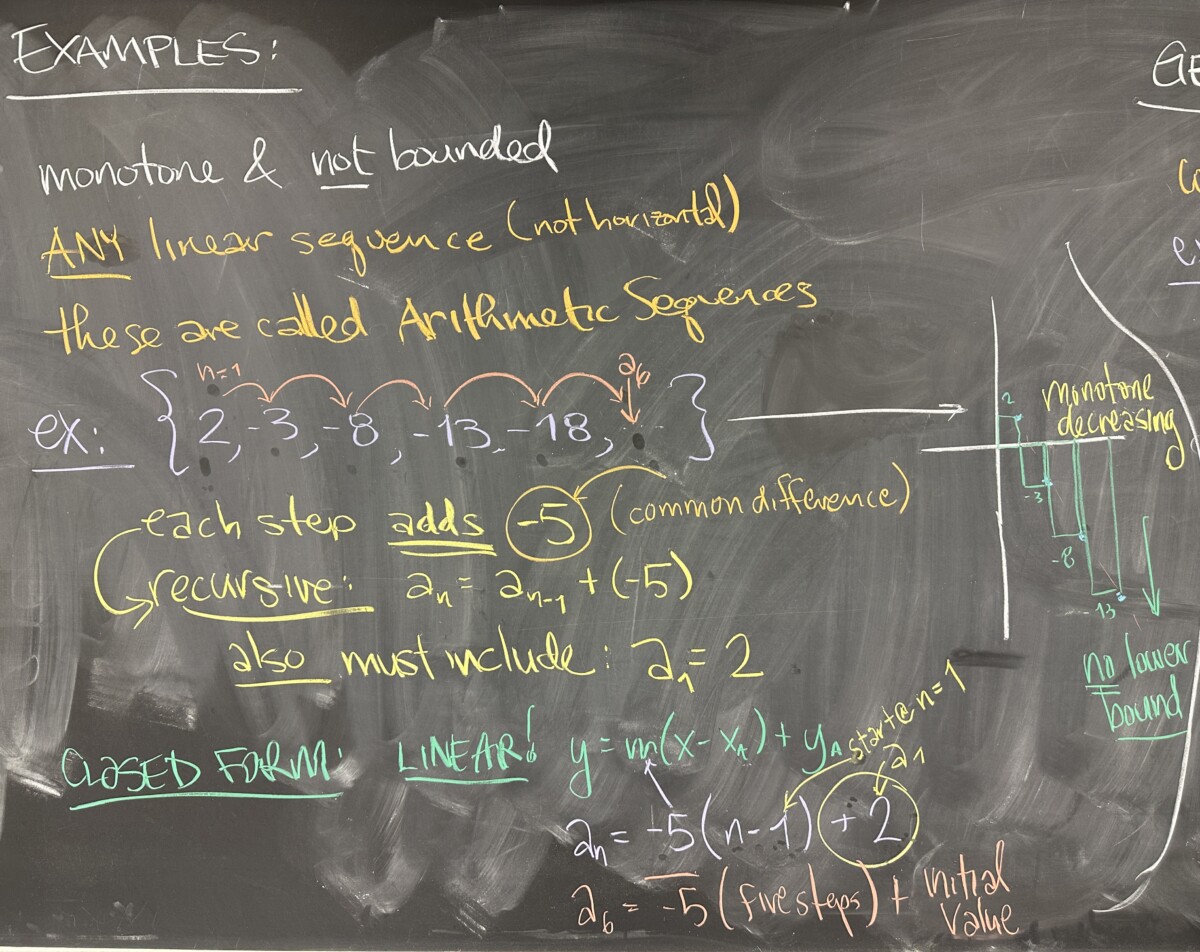
Our first set of examples are “arithmetic” sequences — they have a linear progression. They can be quickly identified because of their “common difference”: any two consecutive terms can be subtracted to get the same value. In this example, \(\{2,-3,-8,-13,-18,\ldots\}\), we see a “common difference” of \(d=-5\) between any two consecutive terms.
Recursively, this means each term is \(-5\) added to its predecessor: \(a_n = a_{n-1} + (-5)\). Now there are lots of other sequences that can be formed by adding \(-5\) over and over again — and they all depend on the “initial term”, the first output value in the sequence. This is the only value that doesn’t have a predecessor! So, in order to completely describe a sequence recursively, we must answer two questions: what is the first term, \(a_1\); and how do we get from one term to the next? In this example: \(a_1 = 2\) and \(a_n=a_{n-1}-5\).
Since “arithmetic” sequences are linear, we can use what we know of linear equations to construct the alternative “closed form” for this example. The “common difference” operates just like slope (they both represent how much the output value changes when the input increases by one), and we have several input/output pairs (for instance \((2,-3),\,(3,-8),\) or \((1,2)\)). It is usually most convenient to always pick \(n=1\) and \(a_1\), both for consistency and because it also emphasizes the importance of the “initial term”, \(a_1\).
When we use the point-slope form for a line, \(y-y_A=m(x-x_A)\), solving for \(y\) and using \(n\) for \(x\) and \(a_n\) for \(y\): \[a_n = d(n-1)+a_1\] \[a_n = -5(n-1)+2\]
Another way to think of it is that the \(n^\text{th}\) term is \(n-1\) steps forward from \(a_1\). Since each step is adding \(d\), that’s a total change of \(d(n-1)\) from \(a_1\). So our conclusion is that \(a_n = d(n-1)+a_1\).
With regards to classification, this example is monotone decreasing (minus five at each step), and it is unbounded. The sequence continues to decrease at a constant rate — meaning that it will always eventually go lower than any bound that you try to find. Because it is not bounded, the sequence cannot converge to any value — it is divergent.
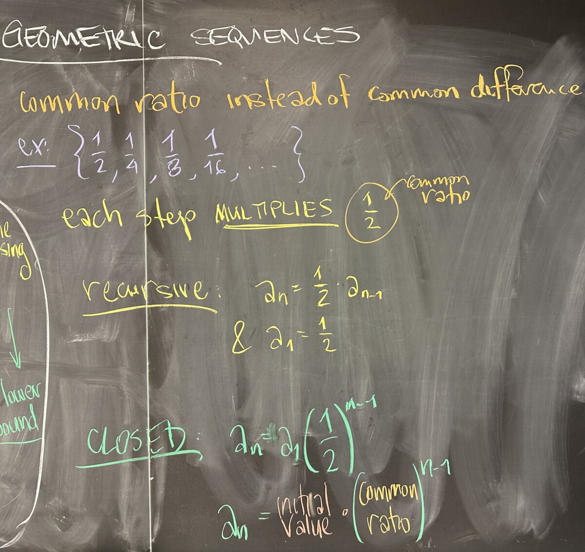
Finally, we get to “geometric” sequences — our first example is one of these! Instead of having a common difference, these sequences have a “common ratio”. Any pair of consecutive terms have a common ratio: \(\frac{a_n}{a_{n-1}}\). In our example, the common ratio is \(\frac12\).
Recursively, we start with \(a_1=\frac12\), and each term is half of its predecessor, so we have \(a_n = \frac12 a_{n-1}\).
If we think of this similarly to the closed form for arithmetic sequences, \(a_n\) is \(n-1\) steps forward from \(a_1\), so that means multiplying \(r=\frac12\) \(n-1\) times, or \((\frac12)^n\), times \(a_1\). This gives us the closed form: \(a_n = a_1(r)^{n-1}\). In our example, this is \(a_n = \frac12\left(\frac12\right)^{n-1}\)


Recent Comments