Definite Integrals

Today’s quiz problem asked about an approximation of the area bounded by the curve $y=x^2-4$ over the interval $[0,2]$ using $n=6$ rectangles.

To start, whenever we’re using the method of Riemann Sums (approximating areas with rectangles), we need to compute $\mathrm{\Delta }x=\frac{b-a}{n}=\frac{2}{4}=\frac{1}{2}$

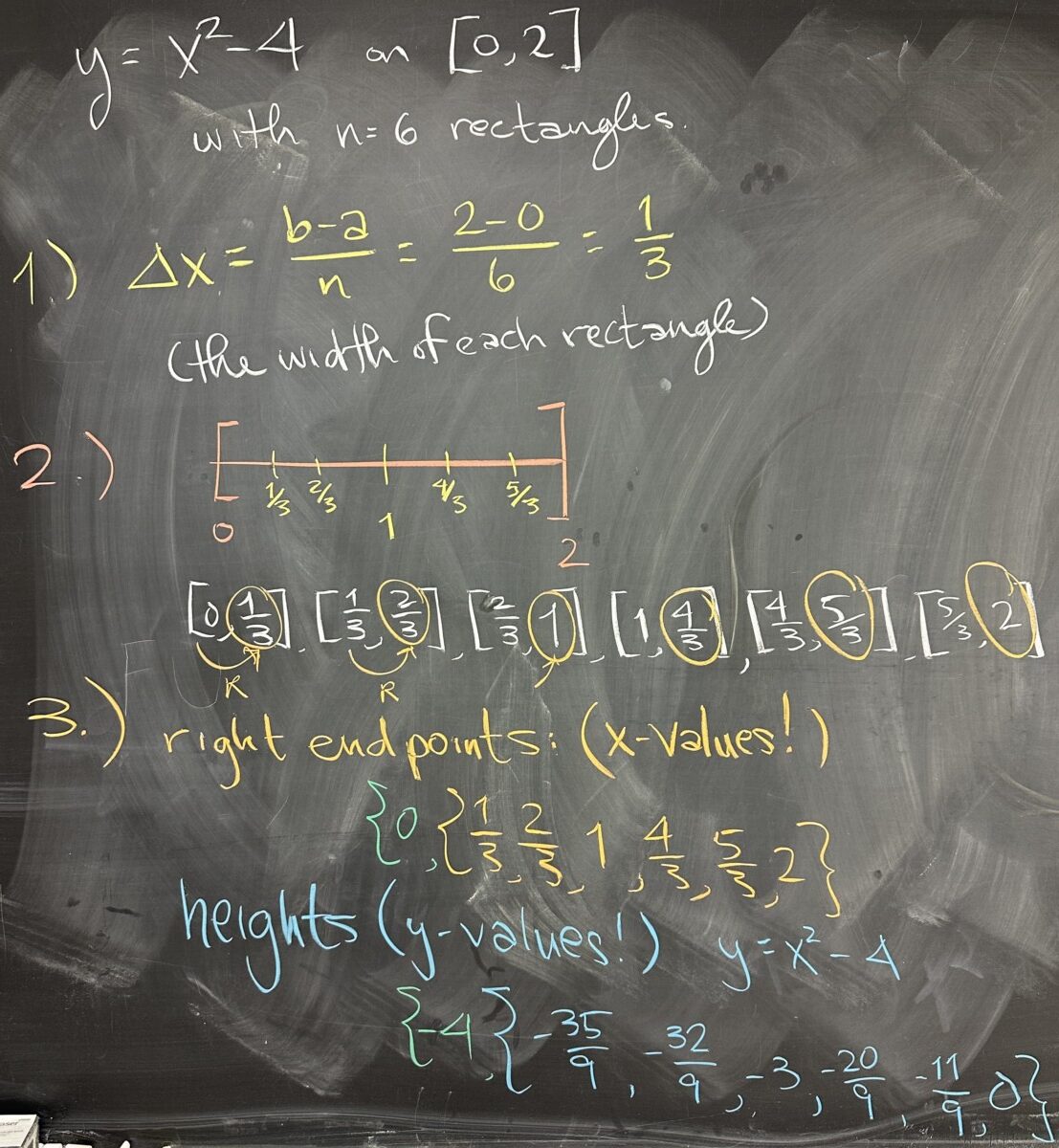
Then, we look at the list of intervals created by splitting $[0,2]$ into $n=6$ sub-intervals with equal width: $[0,\frac{1}{3}],[\frac{1}{3},\frac{2}{3}],[\frac{2}{3},1],[1,\frac{4}{3}],[\frac{4}{3},\frac{5}{3}],[\frac{5}{3},2]$

The problem specifies that we should use the right endpoints: $\{\frac{1}{3},\frac{2}{3},1,\frac{4}{3},\frac{5}{3},2\}$, and from these we compute the heights of each rectangle ($y$-values) by evaluating the $y=x^2-4$ curve at each $x$-value: $\{-\frac{35}{9},-\frac{32}{9},-3,-\frac{20}{9},-\frac{11}{9},0\}$

Now that we have the height of each rectangle, we can compute their areas as $A_i=h_i\cdot \mathrm{\Delta }x$: $\{-\frac{35}{27},-\frac{32}{27},-1,-\frac{20}{27},-\frac{11}{27},0\}$. And then the total area is the sum of the areas of the individual rectangles: $A\approx –\frac{35}{27}+–\frac{32}{27}+–1+–\frac{20}{27}+–\frac{11}{27}+0=-\frac{125}{27}$.

There was a question about process, and we should note here that it is possible to take an alternative approach — summing the heights first, and then multiplying the sum by $\mathrm{\Delta }x$: $(-\frac{35}{9}+–\frac{32}{9}+–3+-\frac{20}{9}+-\frac{11}{9}+0)\frac{1}{3}=-\frac{125}{27}$. This is of course the same total area as multiplying the individual heights by $\mathrm{\Delta }x$ and then taking the sum.

Finally, we are asked about what would be different if we used the left endpoints (instead of the right endpoints). The difference is exchanging the right most $x$-value (and the resulting, right most $y$-value and rectangle area) for the left most $x$-value (and its corresponding $y$-value and area)

• right endpoints ($x$-values): $\{0,\frac{1}{3},\frac{2}{3},1,\frac{4}{3},\frac{5}{3}\}$
• heights ($y$-values): $\{-4,-\frac{35}{9},-\frac{32}{9},-3,-\frac{20}{9},-\frac{11}{9}\}$
• areas: $\{-\frac{4}{3},-\frac{35}{27},-\frac{32}{27},-1,-\frac{20}{27},-\frac{11}{27},0\}$
• total area (for the left approximation): $\frac{4}{3}+–\frac{35}{27}+–\frac{32}{27}+–1+–\frac{20}{27}+–\frac{11}{27}=-\frac{161}{27}$

Although it didn’t get written on the board, we discussed the improved approximation that happens when we use more rectangles (a higher $n$). Although the approximation ends up closer to the actual area, there is also much calculation required. We then proceed without specifying a value for $n$, choosing instead to leave it as a variable.

Without specifying the number of rectangles, the only parameters we need are the curve: $y=f(x)$, and the interval $[a,b]$. We start with the width of each rectangle, by dividing the width of the interval by the number of rectangles: $\mathrm{\Delta }x=\frac{b-a}{n}$.

We then begin listing the $x$-values, each separated by the width of $\mathrm{\Delta }x$: $\{a,a+\mathrm{\Delta }x,a+2\mathrm{\Delta }x,a+3\mathrm{\Delta }x,a+4\mathrm{\Delta }x,\dots ,b\}$. This pattern is familiar, it is arithmetic (with a common difference of $\mathrm{\Delta }x$). Since $n$ already represents the number of rectangles, we need to use $i$ as our index for the pattern of the $x$-values: $x_i=a+i\cdot \mathrm{\Delta }x$, starting with $i=0$.

Then the next step is to find the $y$-values: $y_i=f(x_i)$

And then the areas: $A_i=f(x_i)\cdot \mathrm{\Delta }x$, with a total (approximated) area: $$A\approx \sum _{i=1}^{n}f(x_i)\cdot \mathrm{\Delta }x$$

Then, since the approximation gets closer to the actual area as the number of rectangles, our area is the limit as $n\to \mathrm{\infty }$: $$\underset{n\to \mathrm{\infty }}{lim}(\sum _{i=1}^{n}f(x_i)\mathrm{\Delta }x)$$

The problem is that in order to evaluate this limit, we’d need a closed form for the sum — and this is pretty hard to find, in most cases. Also note what happens to our rectangles as $n\to \mathrm{\infty }$, their width continues to shrink until they’re thinner than the smallest particles in the universe.

Now we introduce some new notation to refer to the exact area: $$A={\int }_a^{b}f(x)dx$$

The $y=f(x)$ and the interval bounds $x=a$ and $x=b$ form the bounds for the region whose area we are trying to find. Also note, in this notation, we have $dx$ taking the place of $\mathrm{\Delta }x$ from our sum. This $dx$ is representative of the infinitesimal width of our rectangles (in the limit as $n\to \mathrm{\infty }$).

Now, for some ‘curves’ (that is to say $y=f(x)$), we can compute the exact area without using the limit of rectangle areas — we can just use geometry instead. In this example, we look at ${\int }_2^{3}2xdx$. By graphing our bounds: $y=2x$ and the interval bounds $x=2$ and $x=3$, we identify the area as a trapezoid. While it is possible to use a formula for the area of a trapezoid, it is perhaps easier to see the total area as the sum of a right triangle on top of a rectangle for a total area of $A=1+4=5$.

This strategy works when $y=f(x)$ is a line, or when $y=f(x)$ is circular. But what can we do when $y=f(x)$ is non-linear?

In our final example, we look at a non-linear curve: $y=x^2$ over the interval $[0,2]$ — and we will use the limit of the rectangular areas to find the exact area of the region.

First, we compute $\mathrm{\Delta }x=\frac{2-0}{n}$, and then the $x$ values by starting with $x_0=0$, and adding the width $\mathrm{\Delta }x=\frac{2}{n}$ to get $x_1=\frac{2}{n}$, then $x_2=\frac{4}{n}$, $x_3=\frac{6}{n}$, and so on.

Knowing this pattern is an arithmetic pattern with common difference $\frac{2}{n}$, we identify the pattern for $x$-values as $x_i=\frac{2}{n}\cdot i$.

From the $x$-values, we compute the $y$-values as $y_i=f(x_i)=(x_i{)}^2={(\frac{2}{n}\cdot i)}^2=\frac{4}{n^2}\cdot i^2$

And then from the heights ($y$-values), we compute the areas: $A_i=y_i\cdot \mathrm{\Delta }x=\frac{4}{n^2}\cdot i^2\cdot \left(\frac{2}{n}\right)=\frac{8}{n^3}\cdot i^2$

So now we are going to try to find a closed form for our sum (so that we can evaluate the limit).

• ${\displaystyle \sum _{i=1}^n\frac{8}{n^3}\cdot i^2}$
• ${\displaystyle =\frac{8}{n^3}\cdot 1^2+\frac{8}{n^3}\cdot 2^2+\frac{8}{n^3}\cdot 3^2+\dots +\frac{8}{n^3}\cdot n^2}$
• ${\displaystyle =\frac{8}{n^3}(1^2+2^2+3^2+\dots +n^2)}$
• ${\displaystyle =\frac{8}{n^3}\left(\frac{n(n+1)(2n+1)}{6}\right)}$

This closed form has the same degree (for $n$) in the numerator and denominator, so the limit as $n\to \mathrm{\infty }$ is the ratio of the leading coefficients: $\frac{16}{6}=\frac{8}{3}$