
Today’s quiz covered the Ratio Test. When using the Ratio Test, we must start by computing \(\displaystyle R=\lim_{n\to\infty}\left|\frac{a_{n+1}}{a_n}\right|\).
Then we must compare \(|R|\) with \(1\).
- If \(|R|<1\), then the series is absolutely convergent.
- If \(|R|=1\), then the Ratio Test is inconclusive.
- If \(|R|>1\), then the series is divergent.

For this series, \(\displaystyle\sum^\infty_{n=1}\frac{n^5}{5^n}\), we have \(a_n=\frac{n^5}{5^n}\), and \(a_{n+1}=\frac{(n+1)^5}{5^{n+1}}\). Then in order to compute \(\lim\frac{a_{n+1}}{a_n}\), we’ll need to divide the fractions by multiplying the reciprocal of \(a_n\). (Note that \(5^{n+1}=5^n\cdot 5\).) \[R=\lim_{n\to\infty}\left|\frac{a_{n+1}}{a_n}\right|=\lim_{n\to\infty}\left|\frac{(n+1)^5}{5^n\cdot5}\cdot\frac{5^n}{n^5}\right|=\lim_{n\to\infty}\frac{(n+1)^5}{5n^5}=\frac15\]
Then, since \(R=\frac15<1\), the Ratio Test tells us that this series converges (absolutely).

The next series, \(\sum\frac{2^n}{n!}\), has \(a_n=\frac{2^n}{n!}\) and \(a_{n+1}=\frac{2^{n+1}}{(n+1)!}\). Again, in order to compute the ratio of consecutive terms, we multiply \(a_{n+1}\) by the reciprocal of \(a_n\). (Similar to the last example, note that \(2^{n+1}=2^n\cdot 2\) and also that \((n+1)!=(n+1)\cdot n!\)) \[R=\lim_{n\to\infty}\left|\frac{2^n\cdot 2}{(n+1)\cdot n!}\cdot\frac{n!}{2^n}\right|=\lim_{n\to\infty}\left|\frac{2}{n+1}\right|=0\]
Then, since \(R=0<1\), the Ratio Test tells us that this series converges (absolutely).

Today we start on a new topic. Our motivating question involves trying to find the distance traveled when speed isn’t constant. While displacement is one measurement of distance traveled, it only works when when traveling in a straight line.
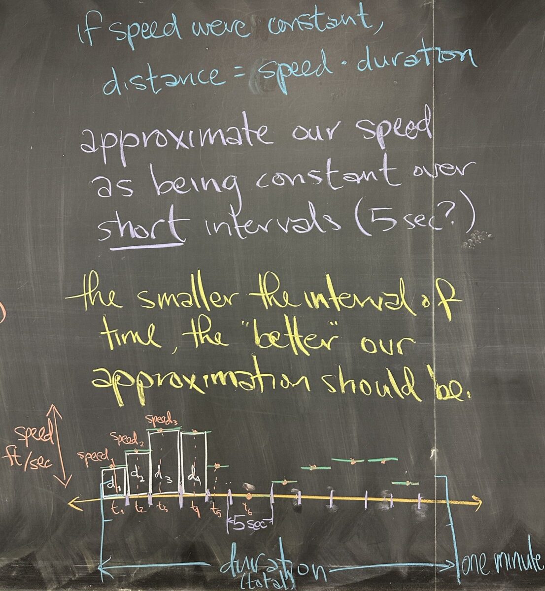
In simpler circumstances, speed might remain constant — in which case, distance traveled can be computed as the product of speed and duration. But for our case, when speed is not constant, we can approximate the distance traveled by treating our speed as constant over very small time intervals. In fact, the shorter the intervals are, the better our approximation will be.
In the illustration, we take the total duration (say one minute), and divide it into five second intervals. On each interval, we treat the speed as constant — multiplying the (assumed) constant speed by the duration of each short interval (five seconds). This product can be visualized as the area of a rectangle with height = speed and width = duration (of the sub-interval, not the total duration). Since each product represents the distance traveled over each short interval, we can add each of these distances to get an approximation of the total distance traveled over the entire duration.

So, the total distance is the sum of the distances over each five-second interval. We can think of this as the sum of products: the speed on each five-second interval multiplied by the five second duration (distance = speed times duration)
Then, if the speed is given by a function (with time as the independent variable), we have \(\text{speed}=f(t)\). The speed on the \(i^\text{th}\) interval is \(\text{speed}_i=f(t_i)\), with \(t_i\) being the time in the \(i^\text{th}\) interval when we measure the speed for the interval.
Then we will denote the duration of the short intervals by \(\Delta t\), in our example, \(\Delta t = 5 \,\text{sec}\). So the approximation of the total distance traveled is \(\sum\left(f(t_i)\cdot\Delta t\right)\).

In general, we treat these problems as approximations of area (although this area might represent something else — as in our earlier example of distance traveled) under a curve described by \(y=f(x)\) over an interval \([a,b]\) (meaning \(a\leq x\leq b\)). In these calculations, we require that the function is continuous on the interval \([a,b]\).
When working out problems like these, we’ll be told how many sub-intervals to use: which we will call \(n\).

The total interval has width \(b-a\), and if we divide it into \(n\) sub-intervals, each will have width \(\Delta x=\frac{b-a}{n}\).
On each sub-interval, we will need a height for our approximating rectangle. Note that each height is a \(y\)-value, and \(y=f(x)\), so we need to choose an \(x\)-value for each sub-interval. There are three ‘common’ ways of choosing these \(x\)-values: the left endpoint, the right endpoint, or the midpoint of each sub-interval.

Moving on to a concrete example, we will approximate the area under the curve \(y=x^2\) over the interval \([0,2]\) using \(n=4\) rectangles.
First we compute the width of each sub-interval. The total width of the interval is \(2\), and with \(n=4\), we have \(\Delta x=\frac24=\frac12\).
Now we take note of the \(x\)-values using \(\Delta x\) on the interval \([0,2]\): \(\{0,\frac12,1,\frac32,2\}\).
If we choose the left-endpoint approximation, our left endpoints are \(\{0,\frac12,1,\frac32\}\).
From each \(x\)-value, we find the height by evaluating the function \(y=x^2\): \[\left\{0^2,\left(\frac12\right)^2,1^2,\left(\frac32\right)^2\right\}=\left\{0,\frac14,1,\frac94\right\}\]

Now that we have the height of each rectangle (and each rectangle has width \(\Delta x=\frac12\)), we can compute the areas: \(\{0\cdot\frac12,\frac14\cdot\frac12,1\cdot\frac12,\frac94\cdot\frac12\}=\{0,\frac18,\frac12,\frac98\}\)
The total area is the sum of the rectangles’ areas: \[0+\frac18+\frac12+\frac98=\frac74\]


Recent Comments