We touched only briefly on the topic of limits at December’s meeting, so I wanted to follow up here. The concept of a limit is absolutely fundamental in a calculus class, but it’s also one that causes the most trouble for students. One possible reason for this is that in most college calculus classes, the formal definition of limit is not even given! The reason that the formal definition is often skipped is that it can look scary to someone who hasn’t seen it before, and it can take a long time to develop an intuitive understanding of what a limit is from the definition. While a tutor will probably never discuss this formal definition with a calculus student, the tutor himself or herself should have an understanding of the formal definition as well as how it implies the intuitive definition we usually give students.

The formal definition

Let f: \mathbb{R} \to \mathbb{R} be a function. We say “\lim_{x \to a} f(x) = L” if for all \varepsilon > 0 there is a \delta >0 such that |f(x) -L| < \varepsilon whenever 0 < |x-a| < \delta.

Quite a mouthful, eh?!

The intuitive definition(s)

We usually say something like, “\lim_{x \to a} f(x) = L means that the closer x gets to a, the closer f(x) gets to L.” Then we usually point at the graph of a function or a table of values of a function and say, “See?!?” This first intuitive definition is not very precise, so why do we think it’s good enough to give to students?

One way to strengthen the intuitive definition is to modify it a little, by adding the key word “arbitrarily” as follows:

\lim_{x \to a} f(x) = L means that f(x) is arbitrarily close to L as long as x is close enough to–but not equal to–a.”

This second intuitive definition might not sound too different from the first intuitive definition, but it’s a way better description of the formal definition above.

From formal to intuitive

One way to understand the formal definition is to try sketching the graph of a function satisfying \lim_{x \to a} f(x) = L and labeling all the components of the definition. This would look something like:

EpsilonDelta0

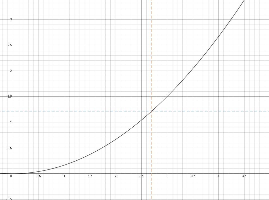
The black curve is the graph of some function f(x), the blue horizontal line is given by y = L and the orange vertical line is given by x=a.

Let’s forget for a second that the formal definition says “for all \varepsilon >0…” and just pick some arbitrary small value for \varepsilon. What does it mean for a y-coordinate of a point to satisfy the inequality |y -L| < \varepsilon? It means that y satisfies -\varepsilon < y-L < \varepsilon, which means that L-\varepsilon < y < L + \varepsilon. Graphically, this means that such a point lies in the blue horizontal band:

EpsilonDelta1

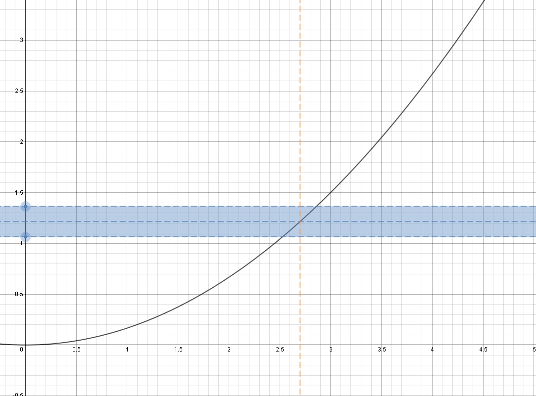
The upper boundary of the blue band is given by y=L+\varepsilon and the lower boundary of is given by y=L-\varepsilon.

The formal definition says that for any \varepsilon >0, we have to be able to find a value \delta > 0 so that if 0 < |x-a| < \delta, then |f(x) -L| < \varepsilon. First, let’s pick a random value for \delta and see what it looks like on the graph:

EpsilonDelta2

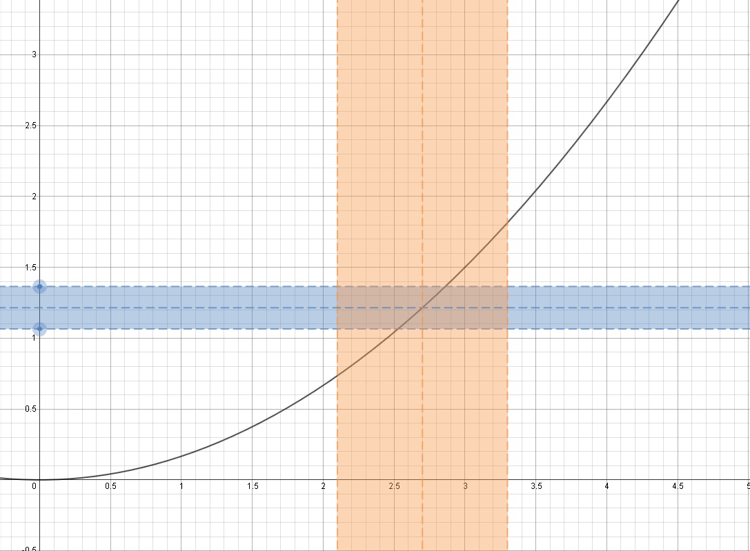
The orange band consists of points whose x-coordinates satisfy |x-a| < \delta. A smaller choice for \delta would make the band skinnier and a larger choice for \delta would make it fatter.

This was just a random choice for the value \delta. Now we can ask if this choice satisfies what we want it to satisfy, namely, if 0 < |x-a| < \delta, is it true that |f(x) -L| < \varepsilon? Graphically, this means we’re asking, “If a point on the black graph is in the orange region, is it in the blue region?” Now it’s clear that the answer is no for this choice of \delta: there are points on the black graph that are in the orange region and not in the blue region. Our first choice of \delta is too big. This is no problem, because we can find a value for \delta that does work; we just have to make it smaller:

EpsilonDelta3

Now every point on the black graph which is in the orange region is also in the blue region. (There are points on the black graph that are in the blue region that aren’t in the orange region, but this doesn’t matter according to the definition.) So what we’ve done is found a particular value of \delta that shows that for our initial choice of \varepsilon, if 0 < |x-a| < \delta, then |f(x) -L| < \varepsilon.

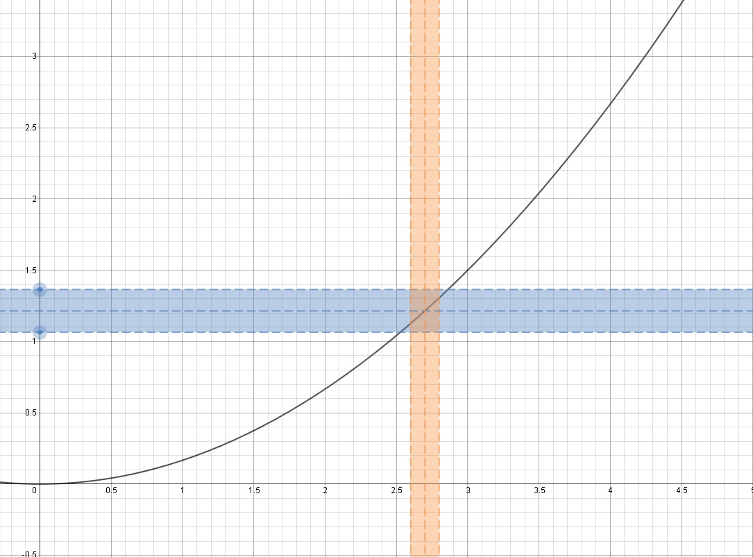
We still haven’t shown that there is such a value for \delta for any choice of \varepsilon>0. We can’t do this formally for every single possible choice for \varepsilon>0, but you can imagine making the blue band around y=L narrower and narrower and trying to find an orange band around x=a that is narrow enough so that every point on the black band which is in the orange region is also in the blue region.

In fact, all the figures above are screenshots from an example in the Desmos catalog; you can play around with different choices of f(x), a, L, \varepsilon, and \delta yourself here!

Now that we have a graphical explanation of the formal definition, we can see that “if we can make the orange band narrow enough so that points on the black graph which are in the orange region are also in the blue region” means that “f(x) is arbitrarily close to L as long as x is close enough to a.” (We also exclude x=a because we don’t care what f(a) is actually equal to.)

Alphabet soup

By the way, \varepsilon is a Greek letter pronounced “EP-sil-on” and \delta is a Greek letter pronounced “DEL-ta.” The formal definition above is known as the “epsilon-delta” definition of a limit.