
The five important points are the x-intercepts and the maximum and minimum points. You should know how to locate them and give their coordinates over one basic period of your function. (If you draw more than one period, you are telling us that you don’t know what “period” means!)
We look at functions whose equations have the form $latex f(x) = a\sin(bx+c)$ or $latex f(x) = a\cos(bx+c)$
The procedure for finding the x-coordinates is the same for all the graphs. The only thing that is different is what the y-coordinate will be: will it be 0 or a maximum or minimum? That depends on whether your function is a sine or a cosine, and also on whether the coefficient a is positive or negative. So the first step is to figure out which basic graph shape your graph should have.
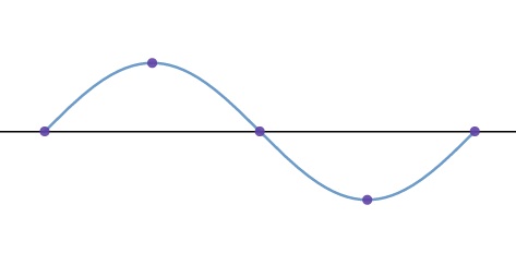
The basic period of a sine function looks like this: The five important points have been marked off in purple dots. Notice that the basic period starts and ends on the x-axis.
Sine with a>0:
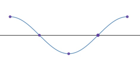
Sine with a<0:

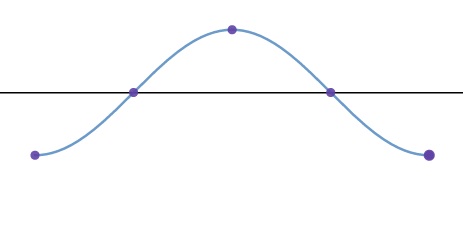
The basic period of a cosine function looks like this: The five important points have been marked off in purple dots. Notice that the basic period starts and ends on either a maximum or a minimum, depending on the sign of a.
Cosine with a>0:
Cosine with a<0:
You just have to keep those general shapes in your mind as you proceed.
First order of business is to find the amplitude, period, and phase shift for your function.
Remember that the amplitude is $latex |a|$ – amplitude is always positive!
The period is $latex \frac{2\pi}{b}$
The phase shift is $latex -\frac{c}{b}$
To find the x-coordinates of the five important points:
• The first point has x-coordinate equal to the phase shift. Mark this x-coordinate lightly with your pen or pencil (don’t put a dot on it, not yet anyway)
• The last point on the basic period (which is the second x-coordinate we find) has x-coordinate equal to the phase shift plus the period. Mark off this x-coordinate lightly with your pen or pencil.
[It is a good thing to keep in mind that the total length you will end up using on the x-axis is going to the one period long! So the distance between the first point and the last point has to be one period. See the picture on p. 246 in the textbook, for example.]
• We will now find the middle x-coordinate. This is halfway between the two ends, so it will be the average of the two x-coordinates we already found. See how I do this in the examples! Mark this lightly – you can do this even before you find it as a number,of course.
• We now find the two remaining x-coordinates: each one is halfway in between two of the points we have marked off so far. Mark them lightly on the x-axis.
• Now we will find the actual points that go with those x-coordinates. That will depend on which of the above four basic shapes of graphs we are dealing with. For the points which are on the x-axis, the y-coordinate is 0. For the points which are maximum points, the y coordinate is the amplitude (positive). For the points which are minimum points, the y coordinate is the negative of the amplitude.
• Now connect the dots with a NICE SMOOTH CURVE (no corners!) to draw your graph. I like to extend the graph a little past the first and last points so that people know the actual graph of the function does not end there.
Here is video slideshow with voiceover showing two examples: These are taken from the textbook, Examples 17.10(a) and 17.10(d). Sorry for the glitch in the second example, which I did not have time to edit.

