Homework Problems taken form Newmann
10.3 Brownian motion
Brownian motion is the motion of a particle, such as a smoke or dust particle, in a gas, as it is buffeted by random collisions with gas molecules. Make a simple computer simulation of such a particle in two dimensions as follows. The particle is confined to a square grid or
lattice L×L squares on a side, so that its position can be represented by two integers i,j = 0… L-1. It starts in the middle of the grid. On each step of the simulation, choose a random direction—up, down, left, or right—and move the particle one step in that direction. This process is called a random walk. The particle is not allowed to move outside the limits of the lattice—if it tries to do so, choose a new random direction to move in.
Write a program to perform a million steps of this process on a lattice with L=101 and make an animation on the screen of the position of the particle. (We choose an odd length for the side of the square so that there is one lattice site exactly in the center.)
Note: The visual package doesn’t always work well with the random package, but if you import functions from visual first, then from random, you should avoid problems.
10.8
Calculate a value for the integral
using the importance sampling formula, Eq. (10.42), with , as follows.
Show that the probability distribution P(x) from which the sample points should be drawn is given by and derive a transformation formula for generating random numbers between zero and one from this distribution. Using your formula, sample N=1,000,000 random points and hence evaluate the integral. You should get a value around 0.84.
10.10 Global minimum of a function
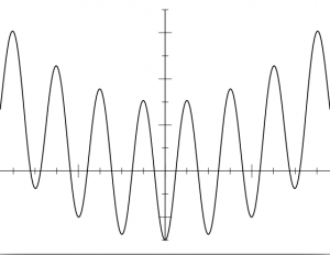
Consider the function , which looks like this:
Clearly the global minimum of this function is at x=0.
Write a program to confirm this fact using simulated annealing starting at, say, x=2, with Monte Carlo moves of the form x →x+δ where δ is a random number drawn from a Gaussian
distribution with mean zero and standard deviation one. (See Section 10.1.6 for a reminder of how to generate Gaussian random numbers.) Use an exponential cooling schedule and adjust the start and end temperatures, as well as the exponential constant, until you find
values that give good answers in reasonable time. Have your program make a plot of the values of x as a function of time during the run and have it print out the final value of x at the end. You will find the plot easier to interpret if you make it using dots rather than lines, with a
statement of the form plot(x,”.”) or similar.
Now adapt your program to find the minimum of the more complicated function in the range 0<x<50.
Hint: The correct answer for part (b) is around x=16, but there are also competing minima around x=2 and x=42 that your program might find. In real-world situations, it is often good enough to find any reasonable solution to a problem, not necessarily the absolute best, so the fact that the program sometimes settles on these other solutions is not necessarily a
bad thing.
10.12 A random point on the surface of the Earth
Suppose you wish to choose a random point on the surface of the Earth. That is, you want to choose a value of the latitude and longitude such that every point on the planet is equally likely to be chosen. In a physics context, this is equivalent to choosing a random vector direction in three-dimensional space (something that one has to do quite often in
physics calculations).
Recall that in spherical coordinates θ,φ the element of solid angle is sinθ dθ dφ and the total solid angle in a whole sphere is 4π. Hence the probability of our point falling in a particular element is
We can break this up into its θ part and its φ part thus:
.
What are the ranges of the variables θ and φ? Verify that the two distributions P(θ) and P(φ) are correctly normalized – they integrate to 1 over the appropriate ranges. Find formulas for generating angles θ and φ drawn from the distributions P(θ) andP(φ). (The φ one is trivial, but the θ one is not.) Write a program that generates a random θ and φ using the formulas you worked out. (Hint: In Python the function acos in the math package returns the arc cosine in radians of a given number.) Modify your program to generate 500 such random points, convert the angles to x,y,z coordinates assuming the radius of the globe is 1, and then visualize the points in three-dimensional space using the \verb|visual| package with small spheres (of radius, say, 0.02). You should end up with a three-dimensional globe spelled out on the screen in random points.


