
Dr. Christopher Blair
BIO 4250
Molecular Evolution & Phylogenetics
Today we will begin working with Bayesian methods to estimate phylogeny and associated evolutionary parameters. Bayesian methods have become extremely popular, partly because they are inherently statistical and allow for a fair degree of flexibility with analyses. Bayesian methods have several similarities with maximum likelihood (ML), particularly through the use of the likelihood function. However, unlike ML, a Bayesian phylogenetic analysis returns an entire posterior distribution of trees and associated parameters (instead of a single ML estimate). There are pros and cons to both methods and often heated debates at scientific meetings and other venues as to which technique is superior. Bayesian analyses require the use of prior distributions on parameters. As the analysis progresses, the prior is updated via the data to return the posterior distribution. How to specify an appropriate prior is one of the most contentious issues in Bayesian phylogenetics (and Bayesian analysis more generally).
We will be working with one of the most popular programs for Bayesian phylogenetics — MrBayes (Huelsenbeck et al. 2001; Ronquist & Huelsenbeck 2003; Ronquist et al. 2012). MrBayes is strictly a command line program, which is useful to prevent researchers from ‘black boxing’ their analyses. Note that MrBayes requires the data to be in NEXUS format. Similar to the ML lab with IQ-TREE, we will first be working with both the 18S animals data set and the vertebrate mtDNA data set. We will once again be performing unpartitioned and partitioned analyses. Make sure that all the input files are in the same directory as the MrBayes executable (mb).
Table of Contents
Bayesian analysis of the animals 18S data set
Our first objective is to estimate a Bayesian phylogeny of the 18S animals data set from your textbook. As MrBayes requires a nexus file as input, I have already converted animals.phy to animals.nexus.
- MrBayes should already be installed on your computer. Your instructor will help you locate the executable. Once MrBayes is loaded, import your data file using the command
exe animals.nexus
- Typing help at the command prompt will bring up a large number of options for analysis. Pay particular attention to the lset and prset commands that control the substitution model and priors respectively. Remember that a major difference between Bayesian and maximum likelihood is that Bayesian methods require priors for all parameters. Typing help lset will show you the current settings and options. For nucleotide data we can set the number of substitutions to 1, 2, or 6. These correspond to some of the more common models we discussed in class. For example, nst =1 would be used under the JC or F81 model that assume a single substitution rate between nucleotides. Conversely, the parameter rich GTR model assumes different substitution rates for each pair of nucleotides, thus we would set nst=6. We can also specify gamma distributed rate heterogeneity and a proportion of invariable sites using the lset command.
Q: How would you specify the K2P substitution model in MrBayes?
After any changes to the model are made, typing
help lset
a second time should illustrate the changes.
A useful new feature of MrBayes is that there is an option that obviates the need to specify a substitution model a priori. Instead, the analysis will sample all of the possible substitution models. In addition, because our sequences are so divergent, we will want to account for different substitution rates across sites. We can do this by adding a parameter for the proportion of invariant sites (I) and gamma (G). Thus, we will specify
lset nst=mixed rates=invgamma
Typing help lset again will allow you to make sure that the changes have been implemented (Fig. 1).
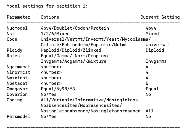
Fig. 1. Model settings for MrBayes. Note that the settings for Nst and Rates have been changed from the default values.
- It’s always a good idea to check the priors before running a Bayesian analysis. In MrBayes, this can be done by typing help prset. As you will see, there are many many options, but the default values here are sensible. Thus, we will not make any changes.
- Before running the analysis, it is good practice to check the model and the parameters to be estimated (Fig. 2).
showmodel
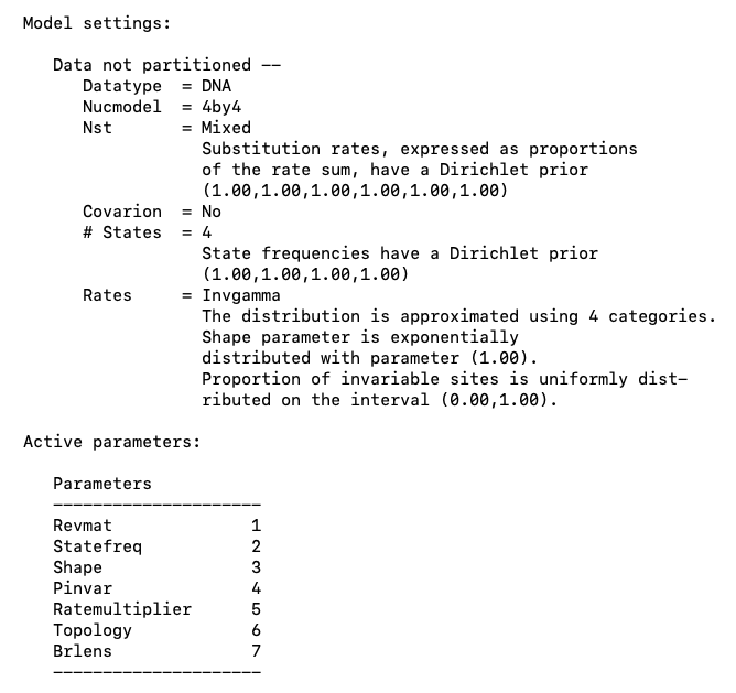
Fig. 2. Current model and active parameters.
Q: How many parameters are in your model? What are they, and what do they mean?
Q: Are we favoring a particular tree topology a priori? How do you know?
- Finally, we need to specify how long we wish to run our analysis. Typing help mcmc will bring up a list of options. The three most important options to be aware of are the following:
Ngen
Nruns
Nchains
Ngen specifies how long to run the analysis. We will use the default of 1 million generations. Nruns specifies how many independent runs we wish to implement. In general, it is good practice to execute multiple independent runs from different starting trees. If the analysis is working well, both independent runs should give us the same answer. If they do not, we may have to spend time troubleshooting. We will use the default of 2 independent runs. Nchains is related to a process called Metropolis Coupling. A value of 4 indicates that each independent run will consist of 4 chains that are sampling parameter values. One chain is what we call the ‘cold chain’ and the remaining chains are ‘heated’. Heated chains can often sample parameter space more efficiently and can help make sure that the cold chain does not get ‘trapped’ in a suboptimal region. The SwapFreq setting specifies how often two chains try to swap states. We will keep the default value of 1. Samplefreq specifies how often the chain is sampled. Let’s change the default value of 500 to 100.
mcmcp samplefreq=100
This means that the analysis will return 1,000,000/100 = 10,000 samples of the posterior which we can summarize.
In any type of Bayesian analysis we want to make sure that we discard samples early on in the analysis. This is because these samples have relatively low likelihood values and we do not want the parameter estimates to bias our analysis. The default settings in MrBayes will discard the first 25% of samples for the cold chain (relburnin=yes, burninfrac=0.25). This is what we will use for our analysis.
- We are now ready to run our first Bayesian phylogenetic analysis! Simply type
mcmc
at the command prompt and the analysis should start. You should see lots of negative numbers on each line (Fig. 3). These represent log likelihood values from each chain. Remember that we implemented 2 runs, each with 4 chains (2 x 4 = 8 total chains). The two runs are separated by the * symbol and the cold chain is indicated by brackets [].
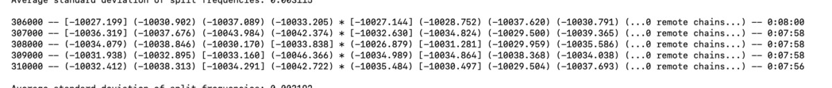
Fig. 3. Example of a MrBayes analysis in progress. This analysis used two independent runs, each with four chains (one cold and three heated).
The analysis should take approximately 10 min to complete. When finished, MrBayes will ask if you wish to continue with the analysis. Before you answer, look closely at the Average standard deviation of split frequencies. This value is an indication of how different your two independent runs are (the smaller the better). To make sure that we have confidence in our results, make sure that this number is <0.01. In my analysis the value is 0.002789. Thus, I will type no into the prompt.
- If you look inside your working directory, you will see that MrBayes output two .p files and two .t files. The .p files are parameter values and the .t files store the phylogenetic trees sampled. We will first summarize the parameters. Type
sump
at the prompt and MrBayes will summarize the results in both .p files. Make sure that 25% of samples are discarded as burnin. If you scroll down, you will see a figure showing generation versus log likelihood (Fig. 4). There should be no obvious trends/patterns in the plot. If there are, you likely need to run the analysis longer.
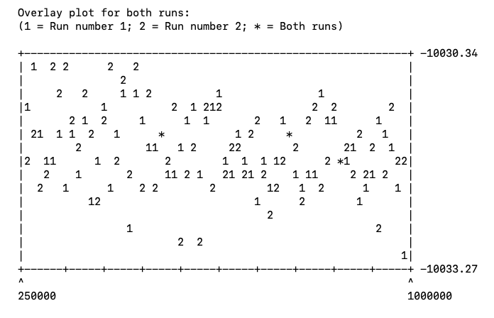
Fig. 4. Diagnosing stationarity in MrBayes. The x-axis represents generation and the y-axis indicates log likelihood. When stationarity is reached there should be no obvious trends in likelihood values.
If you continue to scroll down you will see a table with parameter estimates (Fig. 5).
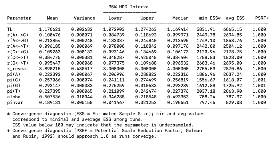
Fig. 5. Parameter estimates from a MrBayes analysis.
Pay attention to ESS and PSRF values. Ideally. We want ESS values > 200 and PSRF values near 1. If this is not the case. We may need to run the analysis for longer. Here, it looks like we are ok.
Q: Look at the list of parameters and their values. Do you know what each parameter represents?
- The final step is to summarize the trees in the .t files. Remember that unlike ML, a Bayesian analysis returns a posterior distribution of trees. In many cases this consists of thousands of alternative trees. Thus, we need some way of summarizing these into one useful summary tree. There are a few ways we could do this. MrBayes generates a majority rule consensus tree. This is a tree where clades occur in >50% of sampled trees (post burnin). Type
sumt
and MrBayes will summarize your trees.
Q: How many total trees are in your .t files?
Q: How many total trees are retained after burnin?
As you scroll down you will see additional information about the analysis. Near the bottom you will see two phylogenies. The first is the majority rule consensus tree with posterior probabilities on nodes. Posterior probability values are a measure of statistical support. In general, values > 95 indicate strong support. Finally, you will see a phylogram with branch lengths measured in expected substitutions per site.
- If you look inside your working directory you should see a file ending in .con.tre. This is your consensus tree from MrBayes. Open this file in FigTree and process the tree similar to what we did for our IQ-TREE analyses.
- Increase the font size for taxon names.
- Root the tree
- Add posterior probability values (Node Labels > Display > prob(percent)
Your phylogeny should look similar to the one below (Fig. 6).
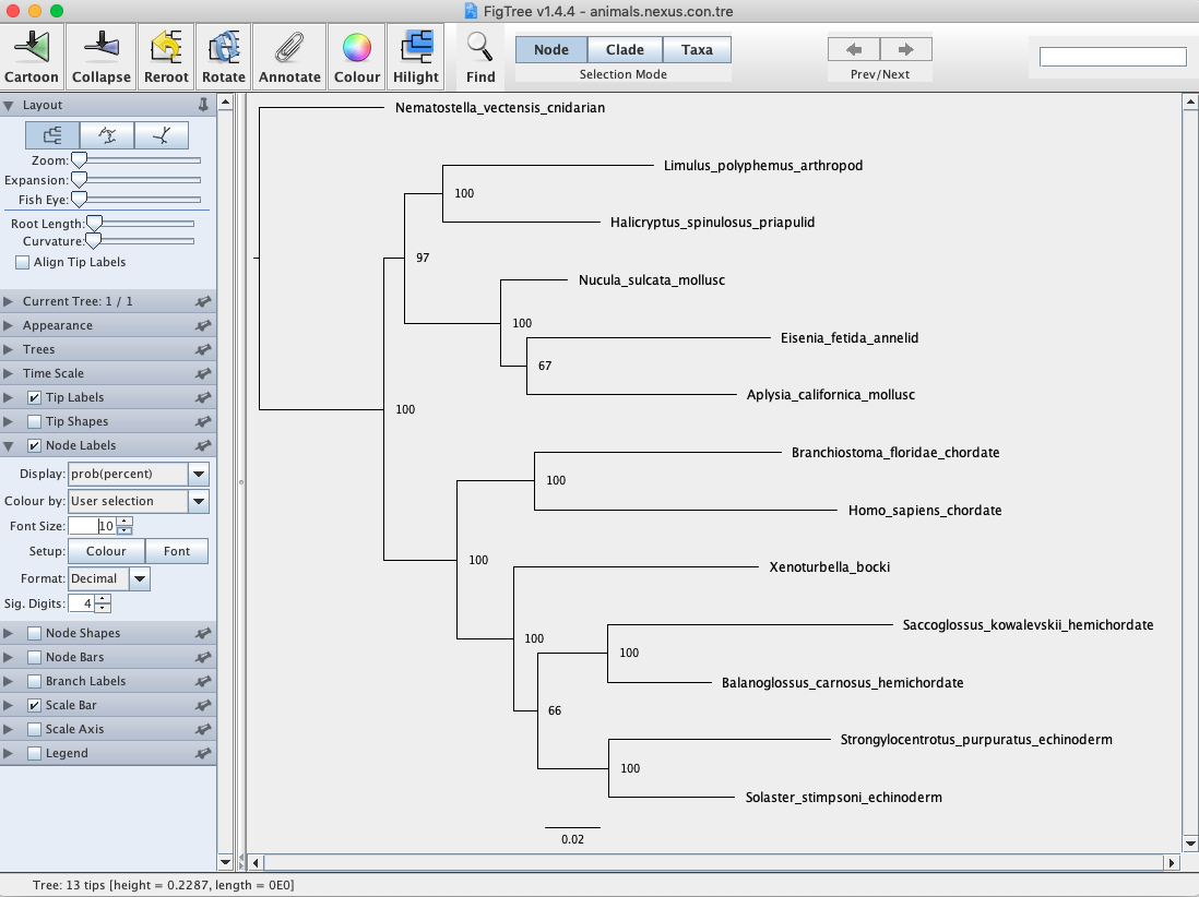
Fig. 6. Bayesian majority rule consensus tree of animal phyla inferred from 18S sequences. Values at nodes represent posterior probability values.
Q: Is your Bayesian phylogeny the same as your ML phylogeny from the previous week?
Q: Does your Bayesian analysis suggest that Xenoturbella is a mollusc?
Bayesian analysis of the vertebrate mtDNA data set
See if you can replicate the steps above to perform a Bayesian phylogenetic analysis of the vertebrate mtDNA data (example2.nexus). Note that we will change some of the analysis settings here. By following the directions above, change Ngen to 500,000, Samplefreq to 50, and Diagnfreq to 1000. Raise your hand if you need help with this. Remember to root the tree using the lungfish. Recall that we also used this data set to estimate a ML tree in IQ-TREE. You should obtain a tree similar to Fig. 7.
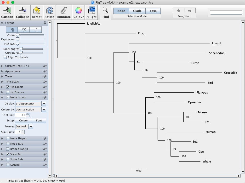
Fig. 7. Bayesian majority rule consensus tree for the vertebrate mtDNA data set. Values on branches represent posterior probability values.
Q: Describe the phylogeny in your own words. What are the major evolutionary findings? Try to use the following words in your description: clade, monophyletic, sister, posterior probability. What relationships are not supported?
Q: How does your Bayesian tree compare to your ML tree you estimated last week?
Partitioned Bayesian analysis of the vertebrate mtDNA data set
Similar to our ML phylogenetic analysis using IQ-TREE, we can perform a partitioned Bayesian analysis in MrBayes. Again, this is useful when analyzing data from multiple genes, combined nucleotide and amino acid data, or combined molecular and morphological data. Note that this can be done by creating a separate text file, by appending a mrbayes block to the data file (common), or by directly typing commands at the MrBayes prompt.
- Open up the file example2-Partitioned.nexus in a text editor and scroll to the bottom. This file is identical to the one we just analyzed, but I have added a mrbayes block that defines partitions. Note that like IQ-TREE, we are specifying three different data partitions and naming the partition scheme ‘mine’. Also note that we are not specifying substitution models for our partitions here. Instead, we will do this in MrBayes.
- Execute example2-Partitioned.nexus
exe example2-Partitioned.nexus
If all goes well, MrBayes should tell you that it successfully read the mrbayes block and recognizes the three partitions (Fig. 8).
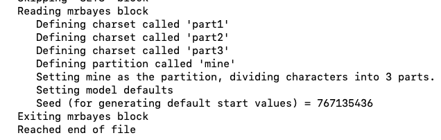
Fig. 8. Text illustrating that MrBayes recognizes the data partitions specified in the input nexus file.
- Typing
showmodel
will show the current analysis settings. Make sure you see information here for all three partitions.
- Our next objective is to specify models for each partitions. We can do this easily using the applyto command. Assume that we want to assign the same model as we did for our unpartitioned analysis.
lset applyto=(1,2,3) nst=mixed rates=invgamma
Typing showmodel again should show the changes.
- Scroll down until you see a table that shows the current parameters to be estimated for each partition (Fig. 9). The same number across partitions indicates that only a single parameter estimate will be made across partitions. For example, in the current settings MrBayes will estimate a single set of state frequencies for Partitions 1-3.
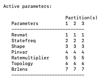
Fig. 9. Current active parameters in a partitioned MrBayes analysis. Note that all parameters are linked across partitions.
Note that we generally want the topology and branch lengths linked among partitions (i.e. we want one topology and set of branch lengths). Conversely, we probably want different model parameters (e.g. alpha, nucleotide substitution rates) for each partition. Thus, we will need to unlink parameters.
unlink statefreq=(all) revmat=(all) shape=(all) pinvar=(all)
If we then type showmodel again we will now see that these parameters are unlinked and MrBayes will estimate each of their values (Fig. 10).
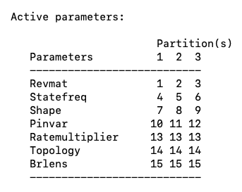
Fig. 10. Current active parameters in a partitioned MrBayes analysis. Note that the parameters Revmat, Statefreq, Shape, and Pinv are now unlinked across partitions.
- Also make sure that you set the evolutionary rates among partitions to variable.
prset applyto = (all) ratepr=variable
as it is highly unlikely that each gene/codon position is evolving at the same rate.
- We should now be ready to run our partitioned Bayesian analysis.
mcmc
- When the analysis finishes summarize the parameters and trees using the sump and sumt commands, respectively.
Q: Did we run the analysis long enough? Why or why not?
- Visualize the tree with posterior probability values (.con file) in FigTree.
Q: Are there any differences between your unpartitioned and partitioned analyses? Explain.
References
Huelsenbeck JP, Ronquist F. 2001. MrBayes: Bayesian inference of phylogeny. Bioinformatics 17, 754-755.
Ronquist F, Huelsenbeck JP. 2003. MrBayes 3: Bayesian phylogenetic inference under mixed models. Bioinformatics 19, 1572-1574.
Ronquist F, Teslenko M, van der Mark P, Ayres DL, Darling A, Höhna S, Larget B, Liu L, Suchard MA, Huelsenbeck JP. 2012. MrBayes 3.2: Efficient Bayesian Phylogenetic Inference and Model Choice Across a Large Model Space. Systematic Biology 61, 539-542.
Print this page
