
Dr. Christopher Blair
BIO 4250
Molecular Evolution & Phylogenetics
In this tutorial you will become familiar with one method used to estimate species trees using multilocus genomic data from next-generation sequencing (NGS) data. The simplest method to estimate a species tree from these data is the traditional concatenation approach (e.g. ML in IQ-TREE), where different gene alignments are combined into one supermatrix. However, concatenation assumes that individual genes share the same history, and thus, the supermatrix approach is not statistically consistent under the multispecies coalescent model. Broadly speaking, we can classify species tree methods into the following categories:
- Fully Bayesian (or likelihood) methods. These methods estimate species trees directly from the sequence data and include StarBEAST2 (Ogilvie et al. 2017), BPP (Flouri et al. 2018), SNAPP (Bryant et al. 2012). Most of these methods can also estimate other parameters such as population sizes and divergence times. Although these methods show relatively decent accuracy, they are extremely computationally demanding and may be of limited use with NGS data sets. However, researchers have been able to run BPP successfully with hundreds to thousands of loci, depending on the analysis.
- Summary statistic (two-step) methods. Summary statistic methods estimate a species tree from estimated gene trees (not the sequence data). Thus, these methods will be sensitive to the accuracy of the reconstructed gene trees, which can be a factor of the data, substitution model, and gene tree reconstruction method. Many of these methods show good accuracy when there is a high degree of incomplete lineage sorting (ILS) in the data, which may be the case with large population sizes and/or short internal branches (i.e. rapid speciation). One of the most popular programs is ASTRAL (Zhang et al. 2018). As the accuracy of these methods depends on the accuracy of gene trees, longer loci are preferred that contain enough phylogenetically informative characters.
- Non-Bayesian methods that estimate species trees from unlinked SNP or multilocus data. The program SVDquartets (Chifman & Kubatko 2014, 2015), estimates a species tree by utilizing observed site pattern frequencies in SNP or multilocus sequence data. As the program does not use Bayesian inference it is quite fast. Benefits over summary statistic methods include the estimation of a species tree directly from the data (versus gene trees). The method does assume a strict clock, but it appears to show decent accuracy even when this assumption is violated. The model is also statistically consistent under the multispecies coalescent model, so is a good choice (versus concatenation) in data sets with a large degree of ILS. SVDquartets is currently one of the best methods (non-likelihood) for estimating species trees with RADseq data.
- Concatenation. Combining multiple gene alignments into one large supermatrix and estimating a species tree from this alignment. Although concatenation assumes that all genes share the same history (i.e. does not account for ILS), it does show good accuracy in many cases. Thus, it is generally recommended to calculate species trees using both concatenation and coalescent-based approaches.
Today we will be estimating species trees using SVDquartets implemented in PAUP* (Swofford 2003).
Link to video tutorial from Bioinformatics BootCamp = https://paup.phylosolutions.com/tutorials/video-tutorials/.
Table of Contents
Species tree analysis in SVDquartets
PAUP* can be run either through a graphical user interface (GUI) or the command line. In this tutorial I will provide instructions for both approaches. The data we will use come from a phylogenomic study on alligator lizards (Blair et al. 2021; Fig. 1). The authors collected thousands of ultraconserved element (UCE) loci (Faircloth et al. 2012) through a technique called target sequence capture. These data were then used to estimate phylogenetic relationships and divergence times. The data also supported the recognition of a new genus (Desertum).
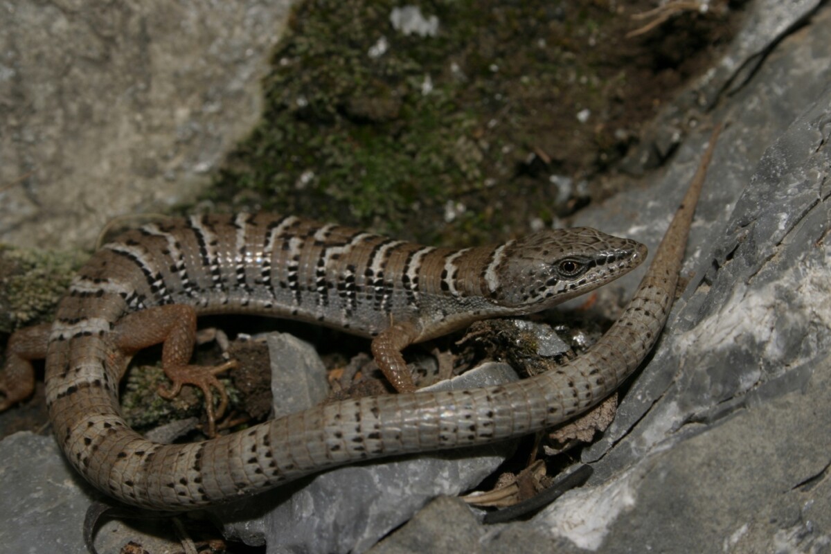
Fig. 1. Pygmy Alligator Lizard (Gerrhonotus parvus). Image credit: Michael Price (https://commons.wikimedia.org/wiki/File:Gerrhonotus_parvus_5880611.jpg). CC BY-SA 4.0.
- Open the data file anguid80_SVDq.nexus in Aliview to get a sense of the sequence data.
Q: How many sequences/individuals are in the data set?
Q: How long is the concatenated alignment? Remember that although SVDquartets takes a concatenated alignment as input, it is considered a coalescent method.
You will likely notice that the taxon names are not very informative. This data set contains multiple individuals for most species. SVDquartets requires that we specify which sequence corresponds with each species through a taxon block.
- Open up the data file in any text editor and scroll to the bottom. You should see a block that contains species names on the left, and sequence ID on the right (Fig. 2). In this example we are calling our taxon partition ‘species’.
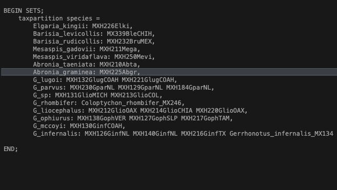
Fig. 2. Assigning individuals to species for species tree analysis using SVDquartets. You can also enter this information directly in PAUP*.
- Open up PAUP* and execute the nexus file
Command line: exe anguid80_SVDq.nexus;
GUI: File > Open
The data set consists of 33 taxa and 1,904,599 characters. A useful feature of SVDquartets is that it allows you to estimate both a lineage tree (using individuals as terminals) and a species tree where individuals are allocated to species. Typing
svdq ?
into the terminal will bring up a list of options. SVDquartets estimates sets of quartet trees (species trees of four taxa) and then combines quartets to estimate the full tree. You can tell PAUP* to evaluate all quartets or a specific number (e.g. 100,000). Obviously evaluating all is more comprehensive, though it may be prohibitive on some larger data sets.
- The first thing we should do is define the outgroup to root our species tree. For this analysis we will use the Madrean alligator lizard, Elgaria kingii, as our outgroup.
Command line: outgroup MXH226Elki;
GUI: Data > Define Outgroup and select sample MXH226Elki
- Let’s try running a species tree analysis using the following command:
Command line: svdq evalQuartets=all nthreads=auto taxpartition=species bootstrap=no;
GUI = Analysis > SVDQuartets and enter the settings shown in Fig. 3.
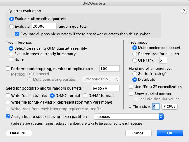
Fig. 3. Setting up a SVDquartets analysis using the graphical user interface (GUI).
When the analysis finishes you should see the SVDquartets tree (Fig. 4).
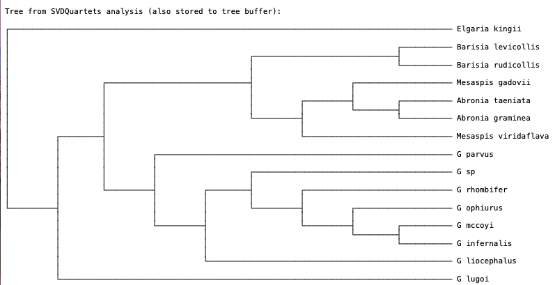
Fig. 4. SVDquartets species tree for anguid lizards.
Q: How many quartets were evaluated?
Q: Are all genera monophyletic? Explain your reasoning. Note that G = Gerrhonotus.
- You can save your species tree using the following:
Command line: savetrees root=yes;
GUI: Trees > Save Trees to File
- The showScores option displays the SVD score for all three unrooted trees for each quartet. Use the command below to display these scores and examine the differences among quartet trees. Remember that the topology with the lowest score is best. To assemble the species tree containing all species, PAUP* uses a quartet assembly algorithm to assemble the species tree based on the quartet trees with the lowest SVD score. See if you can find the best tree for several quartets.
Command line: svdq evalQuartets=all nthreads=auto taxpartition=species bootstrap=no showScores=yes;
GUI: Same as before, but check the box for Show quartet scores.
- Like any type of phylogenetic analysis, we will want to get a sense of uncertainty in the relationships recovered. SVDquartets can use either standard nonparametric bootstrapping or multilocus bootstrapping. For our analysis we will perform standard bootstrapping with 100 replicates.
Command line: svdq evalQuartets=all nthreads=auto taxpartition=species bootstrap=yes showScores=no;
GUI: Uncheck the box for Show quartet scores, and check the box for Perform bootstrapping (make sure 100 is entered).
Note that bootstrapping will take a few minutes. When the analysis finishes you should see two trees (Fig. 5). The first tree represents the SVDquartets tree based on the original data. The second tree is a bootstrap consensus tree. You can think of this as a summary tree of the 100 bootstrap replicates. Researchers have the option to either present the bootstrap consensus tree with support values, or show the SVDquartets tree with bootstrap support mapped on. Note that in many cases the SVDquartets tree is identical to the bootstrap consensus tree.
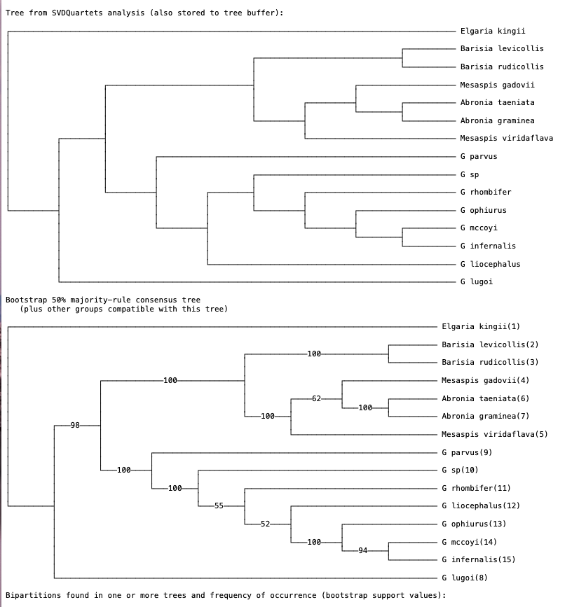
Fig. 5. SVDquartets species tree and bootstrap consensus tree inferred for anguid lizards. Values on branches represent support. In general, bootstrap values >70 indicate moderate-strong support for relationships.
Q: Describe how bootstrapping works in phylogenetic analyses. In our analysis we are using 100 replicates. What does this mean?
Q: Is the SVDquartets tree identical to the bootstrap consensus tree? If not, explain where the differences are.
Q: Does the analysis suggest that a new genus should be erected for G. lugoi? Why or why not?
The GUI version of PAUP* has a cool feature that lets you view and print pdfs of your trees.
Click Trees > Print/View SVDQuartets Trees
Here, you can make edits and export the results for viewing in other programs.
- The previous analysis used a taxpartition block (“species”) to allocate taxa (individuals) to species for estimation of a species tree. Another cool feature of SVDquartets is that it allows you to also estimate a ‘lineage tree’ that is statistically consistent with the multispecies coalescent model. This analysis estimates the phylogenetic relationships of all individual taxa in your matrix. Let’s perform an exhaustive search of all quartets followed by a bootstrap analysis with 100 replicates.
Command line: svdq evalQuartets=all nthreads=auto taxpartition=none bootstrap=yes showScores=no;
GUI: Make sure to uncheck the box for assigning individuals to species.
This analysis will take a bit longer, but should take no more than about 15 minutes. Are bootstrap values high? One benefit of performing a ‘lineage-based’ analysis is that it allows you to test for species monophyly. Note that in many real world studies it can be difficult/challenging to assign individuals to species. Your new SVDquartets tree should resemble Fig. 6.
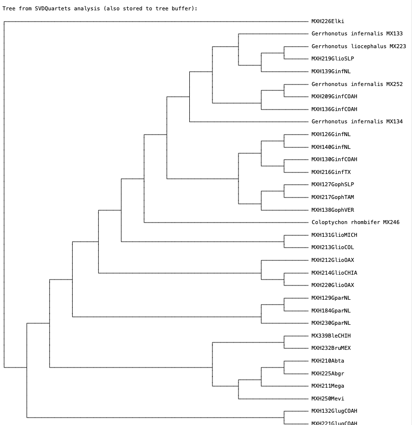
Fig. 6. Lineage-based SVDquartets tree of anguid lizards. Note that in this analysis we are not assigning individual sequences to species. This type of analysis is often helpful for getting a sense of genetic differences between individuals and putative species.
References
Blair C, Bryson RW, García-Vázquez UO, Nieto-Montes de Oca A, Lazcano D, McCormack JE, Klicka J. 2021. Phylogenomics of alligator lizards elucidate diversification patterns across the Mexican Transition Zone and support the recognition of a new genus. Biological Journal of the Linnean Society, blab139.
Bryant D, Bouckaert R, Felsenstein J, Rosenberg NA, RoyChoudhury A. 2012. Inferring species trees directly from biallelic genetic markers: bypassing gene trees in a full coalescent analysis. Molecular Biology and Evolution 29, 1917-1932.
Chifman J, Kubatko L. 2014. Quartet inference from SNP data under the coalescent. Bioinformatics 30, 3317-3324.
Chifman J, Kubatko L. 2015. Identifiability of the unrooted species tree topology under the coalescent model with time-reversible substitution processes, site-specific rate variation, and invariable sites. Journal of Theoretical Biology 374, 35–47.
Faircloth BC, McCormack JE, Crawford NG, Harvey MG, Brumfield RT, Glenn TC. 2012. Ultraconserved elements anchor thousands of genetic markers spanning multiple evolutionary timescales. Systematic Biology 61, 717-726.
Flouri T, Jiao X, Rannala B, Yang Z. 2018. Species tree inference with BPP using genomic sequences and the multispecies coalescent. Molecular Biology and Evolution 35, 2585-2593.
Ogilvie HA, Bouckaert RR, Drummond AJ. 2017. StarBEAST2 brings faster species tree inference and accurate estimates of substitution rates. Molecular Biology and Evolution 34, 2101-2114.
Swofford DL. 2003. PAUP*: phylogenetic analysis using parsimony (*and other methods). Version 4. Sinauer Associates, Sunderland, MA.
Zhang C, Rabiee M, Sayyari E, Mirarab S. 2018. ASTRAL-III: polynomial time species tree reconstruction from partially resolved gene trees. BMC Bioinformatics, 19, 153.
Print this page
