Week 12 – Divergence time estimation

Dr. Christopher Blair

BIO 4250

Molecular Evolution & Phylogenetics

The primary goal of this lab is to use molecular data to estimate evolutionary rates and divergence times. Divergence time estimation is of significant importance to multiple fields of biology ranging from conservation to epidemiology. Unfortunately, some of the theory and methods to estimate rates and divergence times can be a bit abstract and confusing. Several different clock models can be used to estimate divergence times, ranging from a strict clock to an unrooted model where each branch has its own independent evolutionary rate. A strict clock model assumes that each branch on the phylogeny has the same evolutionary rate. This assumption generally holds for closely related species, but is violated when estimating divergence times among distantly related taxa. In such cases, a relaxed clock model (Drummond et al., 2006) may be more appropriate.

Today, we will be working with the software BEAST (Bouckaert et al., 2019), and we will be simultaneously estimating phylogenetic relationships, evolutionary rates, and divergence times. Note that there are multiple ways to incorporate a temporal aspect into phylogenetic analyses to separate rate from time. These include the following:

• Utilize a previously published substitution rate for the gene and group of interest (e.g. 0.02 substitutions per site per million years for avian mtDNA). This is generally the approach when no other information is available. Bayesian methods (like BEAST) allow for uncertainty in the rate estimate by the specification of a parametric prior distribution.

 

• Use fossil information to constrain times of ancestral nodes. Because of the uncertainty in fossil age and fossil placement on phylogenies, Bayesian methods are once again a good choice. Like the rate, uncertainty in fossil age can be incorporated into the analysis through priors. Often, fossils are used to constrain the minimum age of nodes. In other words, the divergence time between two lineages is at least as old as the fossil, but possibly older. A lognormal prior distribution is commonly used.

 

• Use biogeographic information to calibrate nodes. For example, if one fish species occurs on one side of the Isthmus of Panama and its sister species occurs on the other, one can calibrate the ancestral node with the timing of the closure of the Isthmus. This method inherently assumes that divergence or speciation was directly caused by the biogeographic feature, which may often not be the case.

 

• Tip dating can be used for temporal calibration if samples are serially sampled at certain time points. This is a common method to calibrate divergence times in quickly evolving organisms such as viruses.

 

• Secondary calibrations. Nodes can be temporally calibrated based the results from a previous analysis that utilized some of the same taxa. This method is generally discouraged, though can be useful in cases where other techniques are not available.

 

In this lab we will be working with 21 primate TRIM5α sequences (nDNA) from The Phylogenetic Handbook (Lemey et al., 2009). For simplicity we will focus on divergence time estimation using a single gene/locus. However, you should note that in this example we are inferring gene divergence times, which may or may not correspond to species divergence times (the parameter we are usually interested in). Download the NEXUS file (primates.nexus) and open the file in Aliview. Note that the data have already been aligned.

Strict Clock Analysis

It is generally a good rule of thumb to always analyze your data under a strict clock model (and possibly a simple nucleotide substitution model) first to gauge whether you get good mixing and decent effective sample size (ESS) values under the chosen model. Mixing refers to how well the chain samples the posterior distribution, whereas ESS values relate to how many independent samples are used to estimate parameters.

• Open up BEAUti and import your alignment. You can simply click and drag the alignment file into the BEAUti window. Make sure to click the dropdown arrow and select “Import Alignment” (Fig. 1).

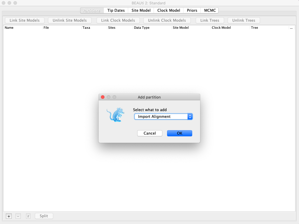
Fig. 1. Importing a multiple sequence alignment into BEAUti.

 

• Click on the Site Model tab and specify the substitution model. For this exercise we will use the GTR+I+G model. Select GTR from the dropdown menu and make sure that base frequencies are estimated. Enter a value of 4 for Gamma Category Count and 0.5 for Proportion Invariant. Finally, make sure the estimate box is checked for both the Shape and Proportion Invariant parameters (Fig. 2).

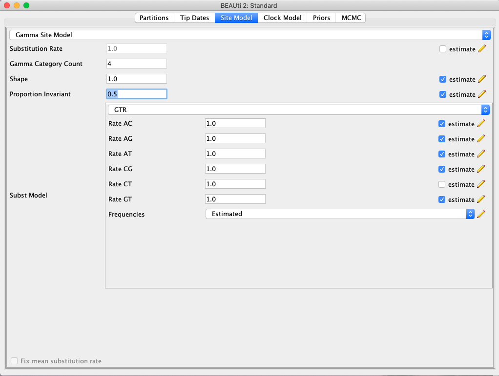
Fig. 2. Selection of a nucleotide substitution model in BEAUti. Here, we are specifying the GTR+I+G model.

 

• Click the Clock Model tab and you will see that a Strict Clock model is set. We will leave this as is for our first analysis.

 

• Now click on the Priors tab where we will setup a temporal calibration. Remember that BEAST is a Bayesian program, and thus all parameters we wish to estimate need priors. There are several published data sets that indicate that humans and chimpanzees diverged approximately 6 million years ago. We will use this information to calibrate the most recent common ancestor (MRCA) of humans and chimpanzees.

 

• Click on the little “+ Add Prior” button to specify a new prior. Name the taxon set anything you wish, and then choose the human and chimp sequences and click the “>>” button.

 

• You should now see a new prior created where we can specify our temporal information. The first thing to do is to click the monophyletic box, so that all sampled trees will group humans and chimps together (Fig. 3).

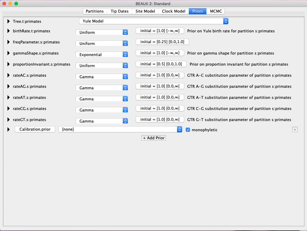
Fig. 3. Setting up priors for Bayesian divergence time estimation in BEAST.

 

• For our temporal calibration, click the center box and select Normal so we can specify a normal distribution for the prior of divergence time between human and chimp. Now click the little black arrow next to our new prior where we can enter a mean and sigma for the normal distribution. We will use a mean of 6 and a sigma of 1.0, which will give us a 95% prior range between 4-8 Mya. Do not change anything else. Go ahead and close this black arrow. If you click on the Clock Model tab you will see that a strict clock is selected and that the estimate box is checked. Because we calibrated the MRCA of chimp and human with a known time, BEAST will be able to provide an estimated substitution rate.

 

• There are a couple more priors to change before we are ready to start the analysis. First, we will change the Tree Prior from a Yule model to a Calibrated Yule Model. Next, change the priors on birthrate and clockRate to a Gamma distribution with an Alpha of 0.001 and Beta of 1000 (Fig. 4).

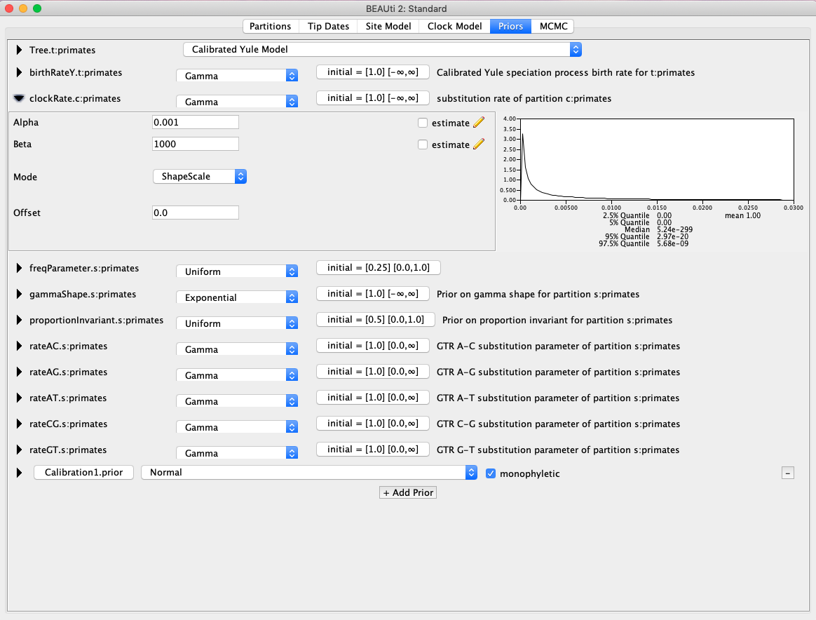
Fig. 4. Changing the prior for the clockRate parameter.

 

• Finally, click the MCMC tab where we can specify the chain length and sampling frequency. For this analysis we will use the default chain length of 10 million generations and sampling frequency of 1000 generations. Click File >Save as and save the xml file. You may need to add the .xml extension. Open BEAST and load your xml file. The analysis should begin and finish in under 10 minutes or so. When the analysis finishes, open the log file in Tracer (Rambaut et al., 2018) to check for adequate mixing and ESS values. Your results should look something like Fig. 5. Click the ‘Trace’ button on the upper right and then click through each parameter. Each trace should look like a ‘hairy caterpillar’ if the chain was mixing well.

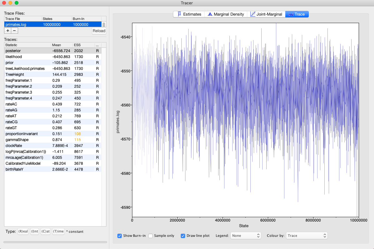
Fig. 5. Tracer results from a Bayesian phylogenetic/divergence time analysis in BEAST. Listed are all parameters estimated by the model. ESS values for two parameters (proportionInvariant, gammaShape) are flagged in yellow because they are <200. Thus, the analysis should be run for a longer duration. Users can also execute two independent BEAST runs and subsequently combine them to increase ESS values.

 

Q: What was the mean rate of evolution of the TRIM5α sequences? What are the units?

 

Q: What was the mean TreeHeight? This is the time of the original divergence at the root node of the tree. What are the units?

 

• Because Tracer suggests that our analysis looks satisfactory, we can now obtain an estimate of phylogeny and associated divergence times. Navigate to your BEAST directory and open TreeAnnotator. Specify a burnin percentage of 10%, maximum clade credibility tree, and mean node heights. Select the primates.trees file from the analysis and name your output file.

Q: What was burnin, and why do we need to use it in Bayesian phylogenetic analysis?

 

• Open up the tree in FigTree where we will add posterior probabilities and 95% highest posterior densities for divergence times. Click on Branch Labels and Display posterior to show posterior probabilities on branches. Now click on Node Bars and Display height 95% HPD. This will show the uncertainty in divergence times for nodes. This obviously is not informative unless we include some type of scale on the tree. Click the box next to Scale Axis and then Reverse axis. Hopefully you have something resembling Fig. 6.

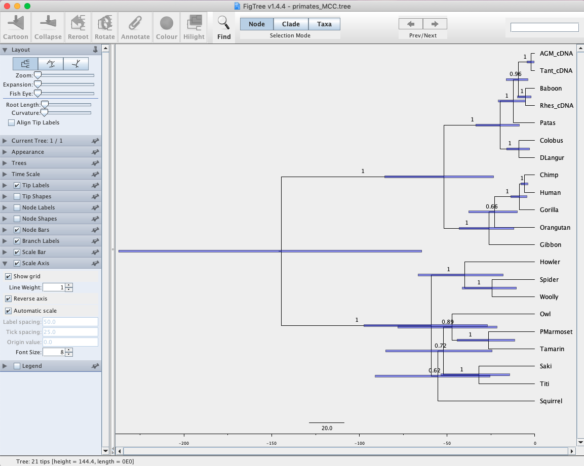
Fig. 6. Maximum clade credibility tree from a Bayesian phylogenetic analysis of primate sequences. Values at nodes represent support values (posterior probabilities). Horizontal bars illustrate 95% HPDs for divergence times.

 

Q: Approximately how long ago did the Howler Monkey diverge from its sister group?

 

Q: Is the major clade that contains human strongly supported? Explain your reasoning.

 

Relaxed Clock Analysis

In the previous analysis we used a strict clock model, which assumes that the rate of evolution is the same across all branches of the phylogeny. A strict clock model is often inappropriate when working with divergent sequences from different species. To determine if a relaxed clock model would fit the primate data better, we will run another BEAST analysis, this time specifying a relaxed clock – lognormal model. All other settings will be identical to our strict clock analysis.

• Go back into BEAUti and click on the Clock Models tab. Change the model from Strict Clock to Relaxed Clock Log Normal. Make sure that the appropriate site model is still specified.

 

• Under the Priors tab set the prior for the ucldMean parameter to a Gamma distribution with alpha = 0.001 and beta = 1000 (Fig. 7). The ucldMean parameter represents the mean evolutionary rate across the tree, explicitly accounting for rate variation among branches/lineages.

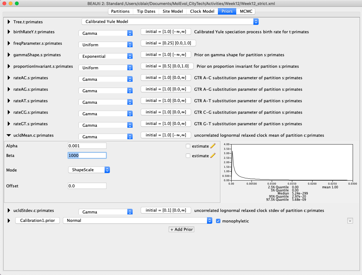
Fig. 7. Changing the prior for the ucldMean parameter in BEAUti.

 

• In the MCMC tab we will once again run the chain for 10 million generations, sampling every 1000. However, change the filename of the log and tree file so that they do not overwrite your previous strict clock analysis. Perhaps something like ‘primates-RelaxedClock.log.’ Save the new xml file and run BEAST again. The analysis should take about 15 min to complete.

 

• When finished, open the log file in Tracer. It may be useful to import the log file for both the strict clock and relaxed clock analyses in the same window to compare parameter estimates (Fig. 8). The first thing to do is make sure all the traces look good and all ESS values are >200. If so, then we know that the analysis has been run for long enough. In this case, ESS vales for two parameters are low. Thus, the best practice would be to run the analysis for longer. However, we will work with these results for the remainder of the tutorial. Take some time to compare parameter estimates between the two analyses. Is there any major conflict that jumps out at you?

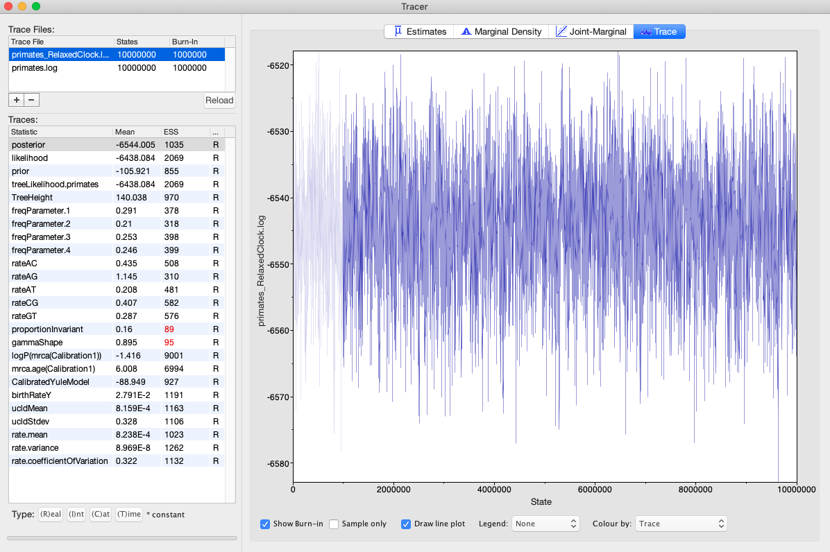
Fig. 8. Trace file for a relaxed clock analysis of the primate sequences in BEAST. Note that ESS values for two parameters are too low, indicating that the analysis should be run longer.

 

Q: How does the ucldMean parameter in the relaxed clock model compare to the clockRate parameter in the strict clock analysis? What does this mean?

 

• Click on the rate.coefficientOfVariation parameter in the relaxed clock analysis. This tells you how clock-like the data are. Values closer to zero provide evidence for a strict clock, whereas higher values signify large branch rate heterogeneity. In general, if 0 is included in the 95% HPD for this parameter we should not reject a strict clock. In other words, we don’t want to overparameterize our analysis.

Q: What are the parameter estimates (mean and 95% HPD) for the rate.coefficientOfVariation parameter? Can we/should we reject a strict clock?

 

• As before, use TreeAnnotator to create a maximum clade credibility (MCC) tree using a burnin value of 10% and mean node heights. Open up this new tree in a new FigTree window to compare to your strict clock tree.

Q: Are the two tree topologies identical? If not, are the differences strongly supported? Remember that Bayesian posterior probability values >.95 indicate strong support.

 

Q: How do the estimated divergence times compare?

 

Q: What are some possible explanations for why the two trees might be so similar?

 

References

Bouckaert R, Vaughan TG, Barido-Sottani J, et al. 2019. BEAST 2.5: An advanced software platform for Bayesian evolutionary analysis. PLoS Computational Biology 15, e1006650.

Drummond AJ, Ho SYW, Phillips MJ, Rambaut A. 2006. Relaxed phylogenetics and dating with confidence. PLoS Biology 4, e88.

Lemey P, Salemi M, Vandamme AM. 2009. The Phylogenetic Handbook: A Practical Approach to Phylogenetic Analysis and Hypothesis Testing, 2nd edition. Cambridge University Press, Cambridge, UK.

Rambaut A, Drummond AJ, Xie D, Baele G, Suchard MA. 2018. Posterior summarization in Bayesian phylogenetics using Tracer 1.7. Systematic Biology 67, 901-904.

Print this page