
In today’s quiz, we tackle the decomposition of a fraction with a denominator that has both an irreducible quadratic factor (\(x^2+9\)) and a repeated linear factor \((x-3)^2\). Here at the start, it is crucial to make sure that we set up the correct decomposition by noting two important signals: the degree of the denominator and the number of factors.
We have a denominator with degree four, which tells us that the decomposition must have four unknowns across the numerators (\(A, B, C, \text{ and } D\)).
We have three factors, which tells us that the decomposition must use three fractions. The numerator for our quadratic denominator must cover the linear and constant terms, while the repeated linear factor will give us two fractions with constant numerators: \[\frac{Ax+B}{x^2+9} + \frac{C}{x-3} + \frac{D}{(x-3)^2} = \frac{x^3-11x^2+15x+63}{(x^2+9)(x-3)^2}\]
After reducing the common denominator across all fractions: \[(Ax+B)(x-3)^2+C(x^2+9)(x-3)+D(x^2+9) = x^3-11x^2+15x+63\]
After expanding all products, we match up the coefficients of each of the like terms to build a system of equations: \[\begin{array}{rcl}1A+0B+1C+0D&=&1\\-6A+1B-3C+1D&=&-11\\9A-6B+9C+0D&=&15\\0A+9B-27C+9D&=&63\end{array}\]
We tried something new for solving larger systems of equations such as this one. Using our calculators, we will put the coefficients into a matrix, with each column corresponding to our unknowns (and a fifth column for the right side of our equations). Using the “rref” function (on our calculators) on this matrix will give us our values for \(A, B, C, \text{ and } D\): \[rref\left(\begin{matrix}1&0&1&0&1\\-6&1&-3&1&-11\\9&-6&9&0&15\\0&9&-27&9&63\end{matrix}\right) = \left[\begin{matrix}1&0&0&0&3\\0&1&0&0&-1\\0&0&1&0&-2\\0&0&0&1&2\end{matrix}\right]\]

Reading one value off of each row, we see that \(A = 3\), \(B=-1\), \(C=-2\), and \(D=2\).
We must now finish the original indefinite integral. After replacing our original fraction with its decomposition, we move to integrate each of the fractions separately. We also should note here that the actual values for \(A, B, C, \text{ and } D\) do not have any impact on our process for integration.
Our first integral \(\int\frac{Ax+B}{x^2+9}\,dx\) needs to be split up before we can continue (because the two pieces each need a different technique): \[\int\frac{Ax+B}{x^2+9}\,dx = A\int\frac{x}{x^2+9}\,dx + B\int\frac{1}{x^2+9}\,dx\]
In the first, we use u-substitution \(u = x^2+9\) and \(du = 2x\,dx\) to conclude \(A\int\frac{x}{x^2+9}\,dx = \frac{A}{2}\ln|x^2+9|\).
In the second, we recognize the pattern for arctangent: \(B\int\frac{1}{x^2+9}\,dx = \frac{B}{3}\arctan\left(\frac{x}{3}\right)\).
The remaining two fractions both use the same u-substitution \(u = x-3\) and \(du = dx\) to conclude that \(C\int\frac{1}{u}\,du = C\ln|x-3|\) and \(D\int u^{-2}\,du = \frac{-D}{x-3}\).
We could have used our values for \(A, B, C, \text{ and } D\) from the beginning, or we can plug them in now for our final answer to the indefinite integral.
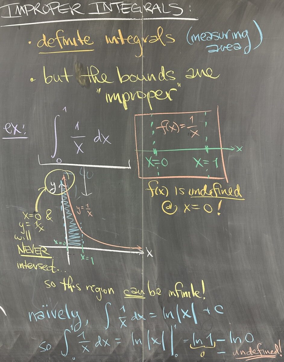
Moving on to today’s topic, we take a look at what are called “improper” integrals. Improper integrals are always definite integrals, but what makes them improper?
Definite integrals are called improper if the function we’re integrating is undefined at one of the bounds for the integral (think \(x=a\) or \(x=b\) with \(f(a)\) or \(f(b)\) undefined). For example, consider \[\int_0^1 \frac{1}{x}\,dx\]
The function, \(f(x)=\frac{1}{x}\), is undefined at the left boundary of the definite integral, \(x=0\) (makes \(f(0)=\frac{1}{0}\), which is undefined). If we consider the graph of this region, we quickly realize that \(y=f(x)\) will never reach the vertical boundary on the left \(x=0\), creating what could be an infinite area!
Naïvely, we may try to just proceed with the Fundamental Theorem of Calculus to compute the area of this region — but that is flawed thinking, because the Fundamental Theorem requires that our \(f(x)\) must be defined on the entire interval \([a,b]\) (in this case \([0,1]\), which \(f(x) = \frac{1}{x}\) is not).
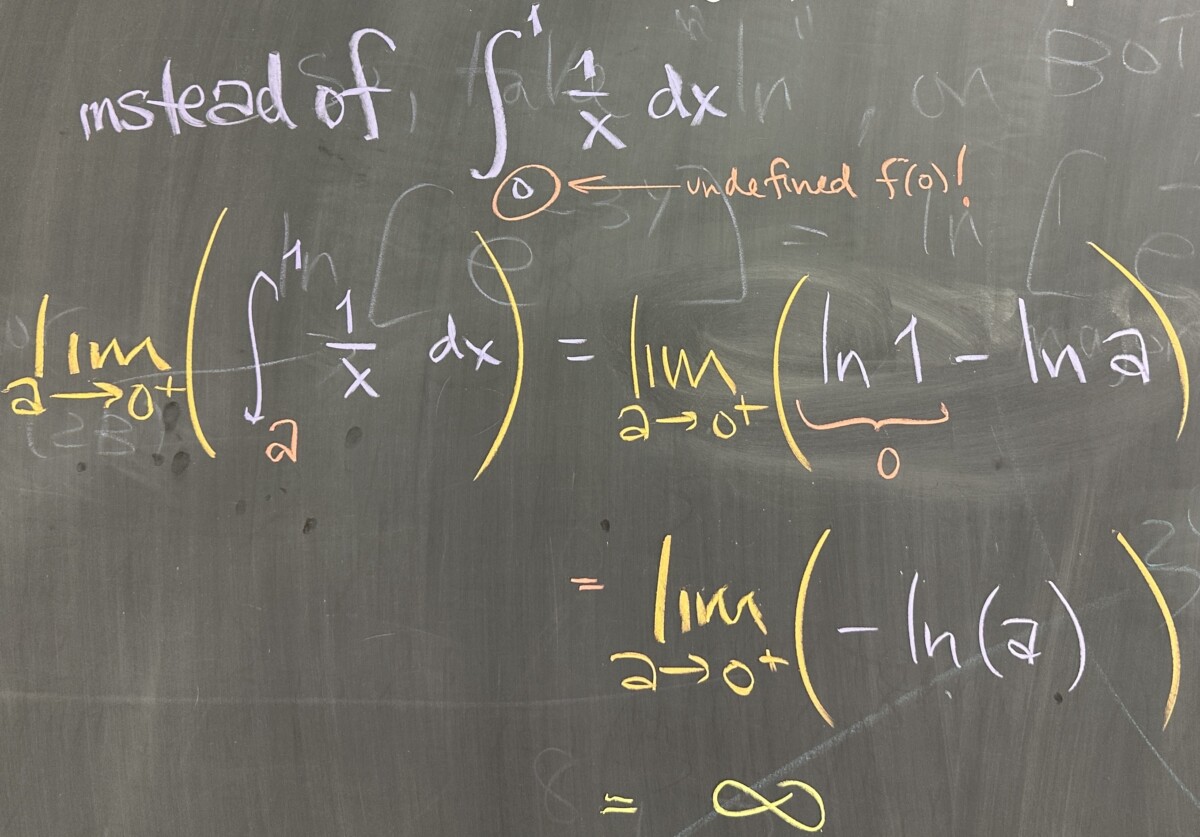
In order to satisfy the requirements of the Fundamental Theorem, we must use a smaller interval on which \(f(x)\) is defined: \([a,1]\) where \(a\) approaches 0 (but doesn’t have to reach 0). Integrating over this smaller interval allows us to use the Fundamental Theorem: \[\lim_{a\to0^+}\left(\int_a^1\frac{1}{x}\,dx\right) = \lim_{a\to0^+}\left(\ln(1) – \ln(a)\right)\]
This limit approaches infinity, so this improper integral “diverges”.
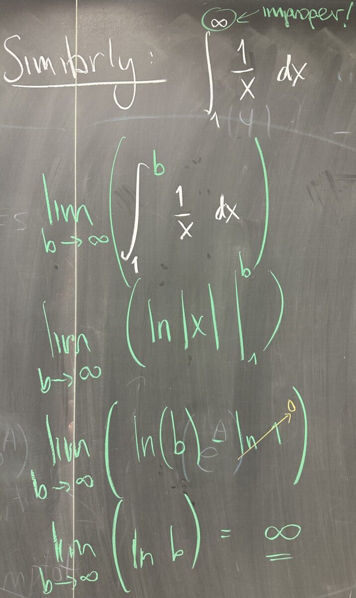
We can also consider what happens if one (or both) of the bounds is (are) infinite. An infinite bound also does not meet the conditions for the Fundamental Theorem and we again use the strategy of a smaller interval. For example, using \([1,b]\) with \(b\) approaching infinity as follows: \[\int_1^\infty \frac{1}{x}\,dx = \lim_{b\to\infty}\left(\int_1^b \frac{1}{x}\,dx\right)\]
Now we can proceed with the Fundamental Theorem: \[\lim_{b\to\infty}\left(\int_1^b \frac{1}{x}\,dx\right) = \lim_{b\to\infty}\left(\ln(b) – \ln(1)\right)\]
This limit is also infinite, so the improper integral “diverges”. It should make sense that \(f(x)=\frac{1}{x}\) has identical behavior for both of these integrals because it is a symmetric function over the line \(y =x\). This means the function has identical behavior between the asymptotes \(x=0\) and \(y = 0\). We see this play out in the fact that both improper integrals for \(f(x)=\frac{1}{x}\) are divergent.
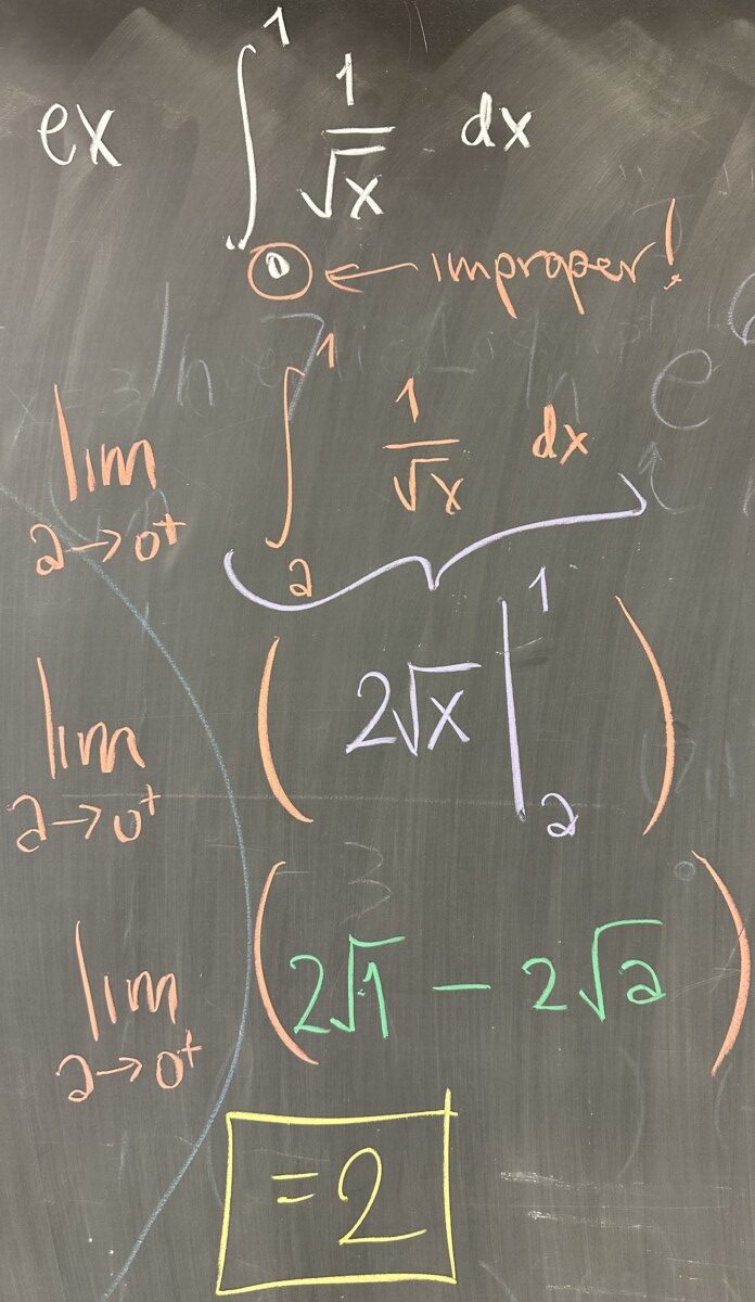
In the next example, we consider \[\int_0^1 \frac{1}{\sqrt{x}}\,dx = \lim_{a\to0^+}\left(\int_a^1\frac{1}{\sqrt{x}}\,dx\right)\]
Using the Fundamental Theorem: \[\lim_{a\to0^+}\left(\int_a^1\frac{1}{\sqrt{x}}\,dx\right) = \lim_{a\to0^+}\left(2\sqrt{1}-2\sqrt{a}\right) = 2\]
This definite integral has finite area, so the improper integral is convergent (to \(2\)).
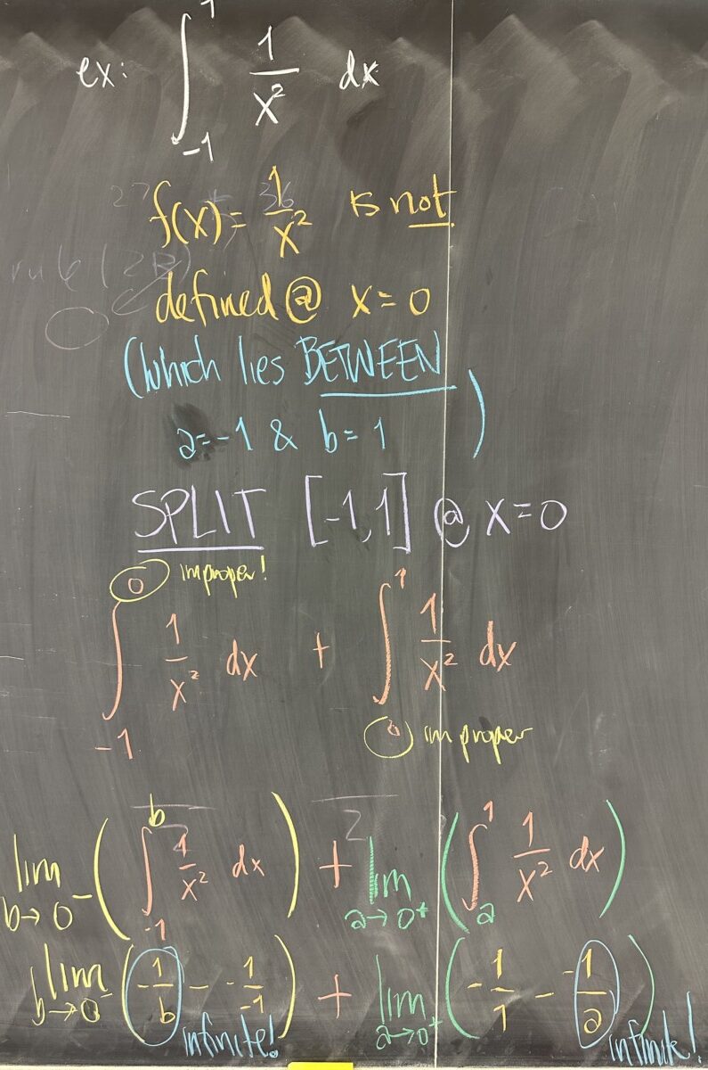
In our final example, we look at a rather sneaky improper integral. Everything looks okay with \(\int_{-1}^1\frac{1}{x^2}\,dx\) until we realize that \(f(x)=\frac{1}{x^2}\) is not defined at \(x=0\) — which is contained in our interval \([-1,1]\)!
Because of this “hole” in the domain of \(f(x)\), we must split the interval into two pieces: \([-1,b]\) and \([a,1]\) (with \(b<0\) and \(a>0\)). Remember that because of the requirements for the Fundamental Theorem, we must use closed intervals where \(f(x)\) is defined. By letting both \(a\) and \(b\) approach \(0\), we will determine whether this improper integral converges or diverges.
For the left interval: \[\lim_{b\to0^-}\left(\int_{-1}^b\frac{1}{x^2}\,dx\right) = \lim_{b\to0^-}\left(\frac{-1}{b} – \frac{-1}{-1}\right)\]
This limit is infinite, so the entire definite integral must diverge. For completeness, we also consider the right interval: \[\lim_{a\to0^+}\left(\int_{a}^1\frac{1}{x^2}\,dx\right) = \lim_{a\to0^+}\left(\frac{-1}{1} – \frac{-1}{a}\right)\]
This limit is also infinite, which makes sense because \(f(x) = \frac{1}{x^2}\) has “even” symmetry (across the \(y\)-axis). This means that the area of the region to the left of the \(y\)-axis should mirror that of the region to the right of the \(y\)-axis.


Recent Comments