Today’s lesson started with students requesting to see problems from the Exam 1 Review sheet. We did several before proceeding to talk about the new unit — what will come after Exam 1.
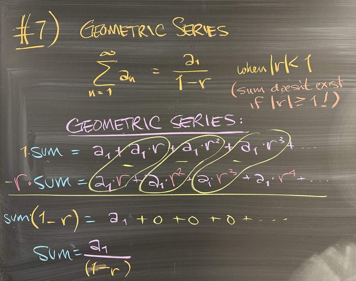
We started by talking about the sums in problem 7. Each of these is a geometric series — which are the only series (that we talked about) where the value of the infinite sum is known. We have discussed the formula \[\sum^\infty = \frac{a}{1-r}\] where \(a\) is the first term of the series and \(r\) is the common ratio — but we had never gone over why this is true.
All geometric series have the form \(a + ar + ar^2 + ar^3 + \ldots\), so with some clever work, we can deduce that if \(S\) represents the (unknown for now) value of the infinite sum, then \(S(1-r) = a\), which can be solved for \(S = \frac{a}{1-r}\).
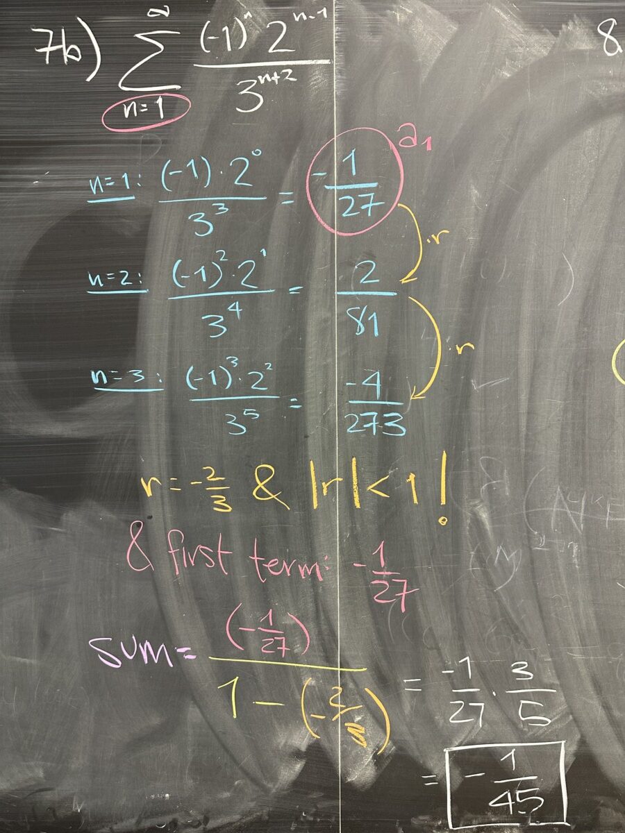
In problem 7b, we apply this knowledge. We don’t have to identify these values directly from the formula \(a_n = \frac{(-1)^n2^{n-1}}{3^{n+2}}\). Writing out the first few terms helps us establish values for both \(a\) and \(r\).
Once we have those two values, the sum is found by substituting \(a = -\frac{1}{27}\) and \(r = -\frac{2}{3}\). Then we do some arithmetic to simplify the result.
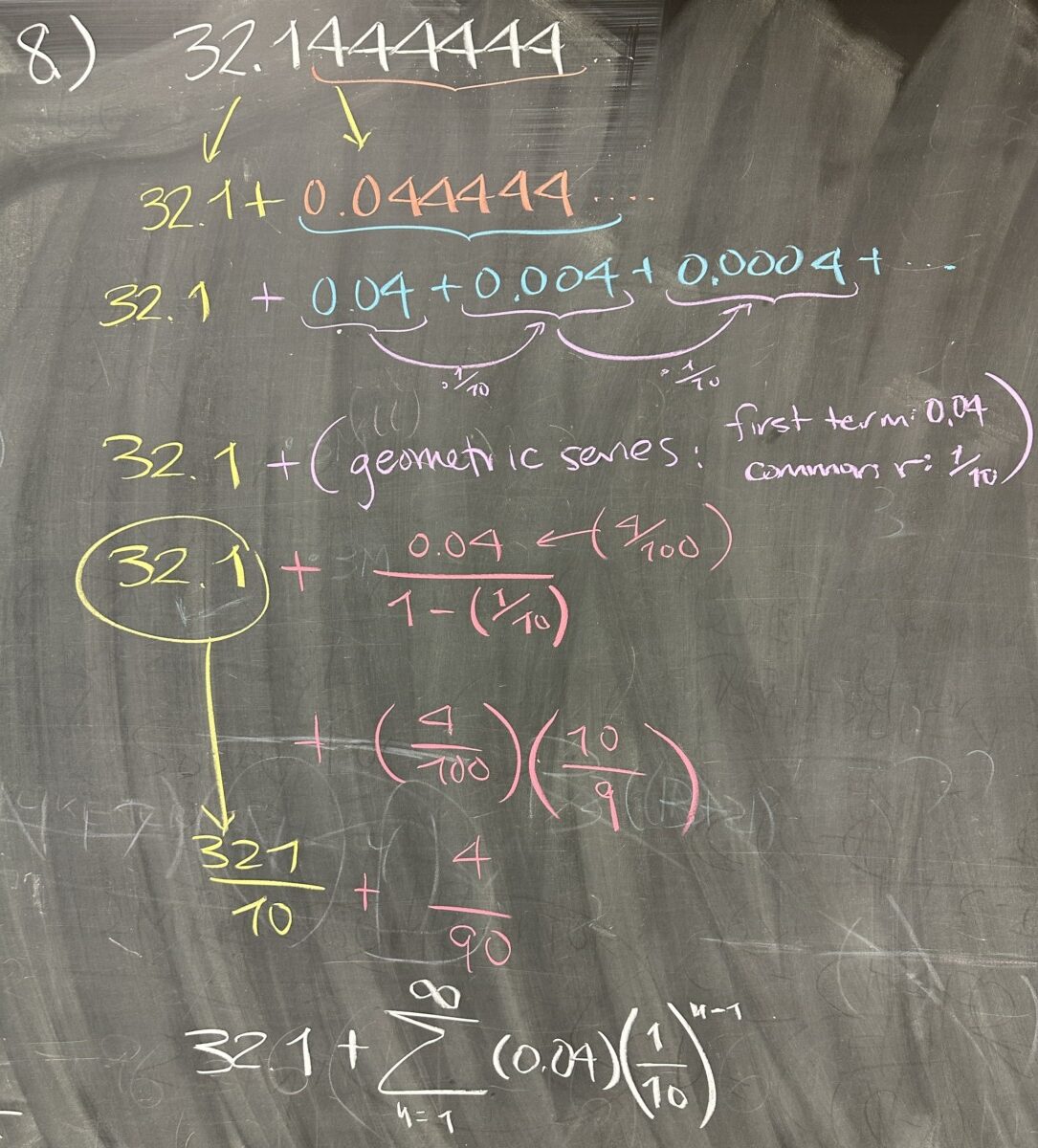
Problem 8 is also a geometric series problem. The real trick is knowing how to write the repeating decimal as a geometric series. Find where the pattern starts and then write it as a repeating sum. Once we do the first two or three terms, it is easy to identify the first term, and then the common ratio.
Knowing those two pieces of information, we can use the formula \(S = \frac{a}{1-r}\) to write the repeating part of the decimal as a single fraction. The non-repeating portion at the beginning, \(32.1\), can also be written as a fraction, \(\frac{321}{10}\). We didn’t combine them here, but the sum would be \( \frac{321 \cdot 9}{10\cdot 9}+\frac{4}{90} = \frac{2889+4}{90} = \frac{2893}{90}\).
You can check this work by dividing \(2893\) by \(90\) to see what decimal that gives.
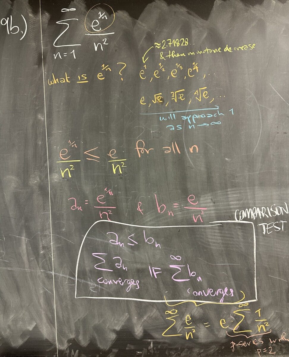
We did 9b, a convergence test question. The numerator \(e^{1/n}\) was a bit confusing for everyone, so we looked at its pattern: \[\left\{e \approx 2.718, e^{1/2} = \sqrt{e} \approx 1.648, e^{1/3} \approx 1.396, e^{1/4} \approx 1.284, \ldots \right\}\] This pattern represents higher and higher roots of \(e\), which is a monotone decreasing pattern with limit 1.
Regardless, we can see that this pattern will always produce numbers less than (or equal to, in the case of \(n=1\)) the number \(e\).
As a result, we know that our sequence \(a_n \leq \frac{e}{n^2}\), so our series must be \(\displaystyle\sum^\infty a_n \leq \sum^\infty \frac{e}{n^2}\). And because \(e\) is a constant, it can be factored out of the series, leaving us to determine the convergence or divergence of \(\displaystyle\sum^\infty \frac{1}{n^2}\). We know this series is convergent because it is a p-series with \(p = 2 > 1\).
By Direct Comparison Test, our series is less than a convergent series. And because all of our terms are positive, the sum must monotone increase as n grows to infinity. Our series is bounded by the larger convergent series and monotone — therefore it must also converge.
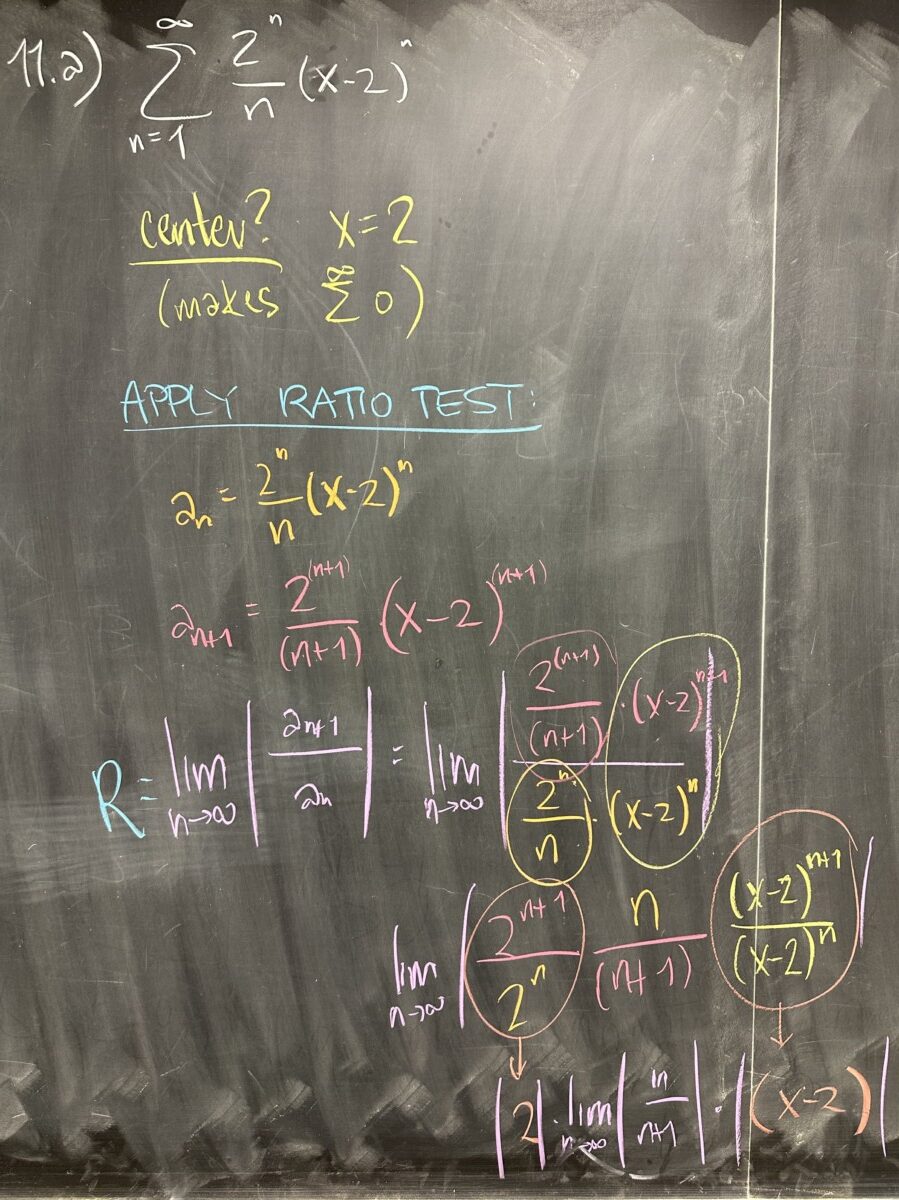
Finally, we did a power series problem. The first thing we did was to identify the \(x\)-value that causes the series to be the sum of zeros, \(x = 2\).
Whenever we are looking to find an interval of convergence, we use the Ratio Test. Here, we computed the limit of the ratio of consecutive terms to be \(2|x-2|\).
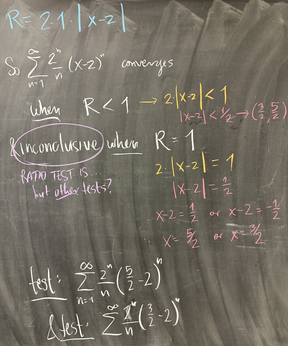
The Ratio Test tells us that our series converges so long as this limit is strictly less than one. The Ratio Test is also inconclusive when this limit equals one.
Both of these facts lead us to \(x = \frac{5}{2}\) and \(x = \frac{3}{2}\) as the endpoints of our interval. The Ratio Test is inconclusive at these endpoints, so we will need to use other tests — which is no problem, we have plenty!
We did not complete this problem for lack of time, but you should simplify the series at each endpoint. You should find that one of them is a p-series, and the other is an alternating series. Use the corresponding tests to determine convergence at each endpoint.
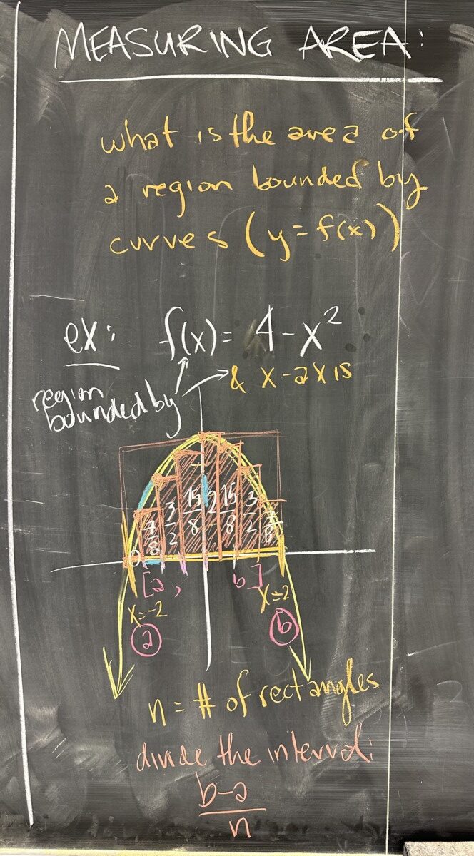
One of the fundamental questions we will tackle in Calculus II is the question of area enclosed by curves. Our example here asks for the region bounded by \(f(x) = 4 – x^2\) and the \(x\)axis.
In order to answer this question, we will use a shape whose area we know quite well: the rectangle.
We start by identifying the range of \(x\)-values that the area includes. For us, that is the interval \(x \in [-2,2]\). We then break that interval into smaller intervals. The smaller the pieces we break it into, the closer our approximation will be. In our example, we opted for \(n = 8\) rectangles.
As a result, since our original interval is \(4\) units wide, each rectangle will be one-eighth of that.
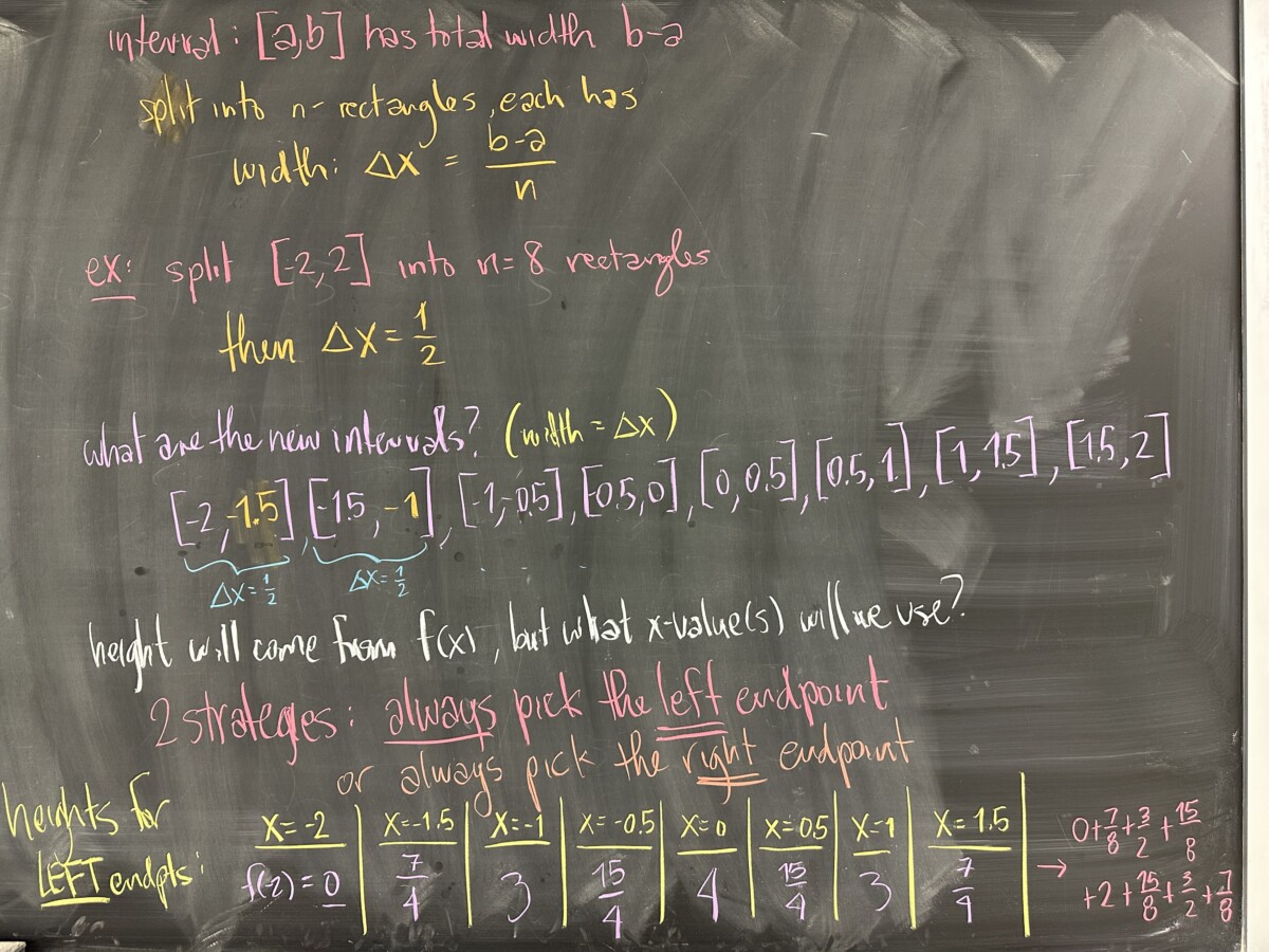
We call the width of each of the smaller intervals \(\Delta x\). In our case \(\Delta x = \frac{4}{8} = \frac{1}{2}\).
With our new width in mind, we start listing the sub-intervals starting from the left endpoint, \(x = -2\). Once we do \(8\) intervals, we finally arrive at our right endpoint, \(x = 2\).
Each of these sub-intervals will represent the width of a rectangle, and they each have the same \(0.5\) width.
What about the height of each rectangle? Well, height is measured in the \(y\) direction, and we have \(y = f(x)\). So we must pick an \(x\)-value from each of our sub-intervals and plug it into our function to get a \(y\)-value that we can use for height.
To start out with, we will be using two strategies:
- always pick the left endpoint of the sub-interval
- always pick the right endpoint of the sub-interval
- (you could also pick the midpoint of the sub-interval, but that requires yet another round of calculations!)
If we go for the “left endpoint” strategy, we listed the left endpoints (in yellow) and then computed the corresponding \(y\)-value for each. With these heights in hand, we only needed to multiply each by the width (remember each width is \(0.5\)) to get the areas of each of the eight rectangles.


Recent Comments