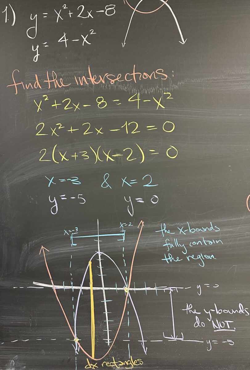
Today’s quiz consisted of several questions centered around finding the area between two curves: \(y=x^2+2x-8\) and \(y = 4-x^2\). The first question asked for the points of intersection for the two curves. By substitution, we arrive at \(x^2+2x-8=4-x^2\) which has solutions \(x=-3\) and \(x=2\). In order to find the points of intersection, we need both \(x\) and \(y\)-coordinates, so for each \(x\) we find the corresponding \(y\). Note that our two \(x\)-values are intersections of the two curves, so both equations should give us the same \(y\)-value when we plug in the same \(x\)-value.
We find then that our two intersection points are \((-3,-5)\) and \((2,0)\). If we then graph our two curves (each is a parabola, so we can identify the vertex of each one), we arrive at the image shown in the photo. Note here that the intervals for \(x\) and \(y\) are illustrated. The \(x\)-values from the intersections form an interval which fully contains the region enclosed by the two curves (in other words, the region does not extend to the left of \(x=-3\) nor to the right of \(x=2\).
On the other hand, the \(y\)-values from the intersections form an interval that does not contain the region. The region extends beyond (above) \(y=0\) and also extends below \(y=-5\). This means that our intersection points do not give us a good interval for \(y\), but we do have a good interval for \(x\). As a result, we will choose to proceed with this problem using “dx” rectangles (as illustrated by the narrow orange rectangle).
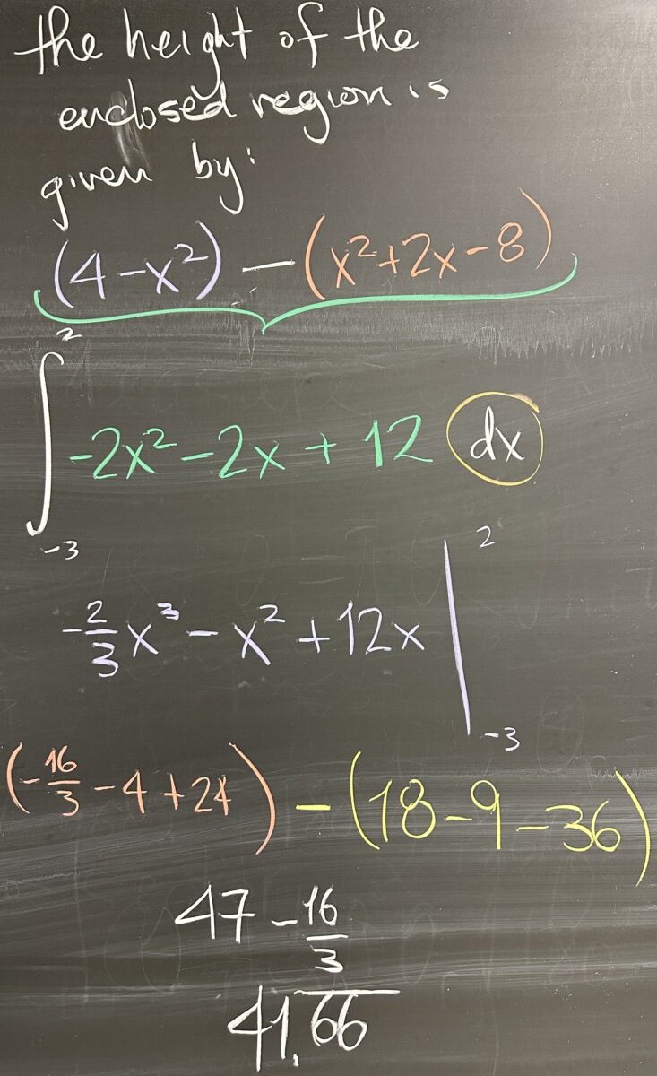
Once we know the intersection points, and have identified the intervals and decided whether to use “dx” or “dy” rectangles, we then proceed to find a function that describes the height of our region. (Note that if we were using “dy” rectangles, we would instead need to find a function for the width of our region.)
In either case, we must determine which of the two curves is “greater” on the interval for the region. Since we have the interval \(-3 \leq x \leq 2\), we may choose any \(x\)-value from the interval to determine which curve is larger — so choose something easy like \(x=0\). The first curve \(y = x^2+2x-8\) has \(y=-8\) when \(x=0\), and the second curve \(y = 4-x^2\) has \(y=4\) when \(x=0\). Since \(y=4\) is greater than \(y=-8\), the second curve is “greater” and our height function is given by the greater curve minus the lesser curve: \[(4-x^2)-(x^2+2x-8) = -2x^2-2x+12\]
Finally, we integrate the height function over the interval: \[\int_{-3}^2 -2x^2-2x+12\,dx = \frac{125}{3}\]
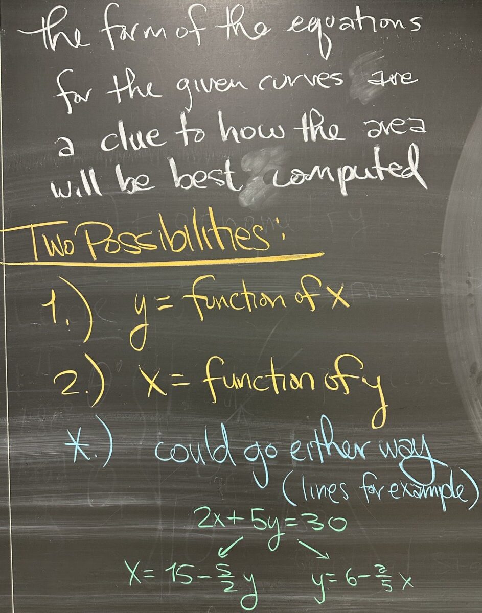
There is a general strategy when considering regions bounded by intersecting curves. Their form can give us useful information — and there are two possibilities. Either the equation for the curve can be solved for \(x\), or for \(y\) (or both — is that a third possibility?)
In cases where the curves can be represented as \(y=f(x)\), we will be inclined to use \(dx\) rectangles, with bounds for \(x\). Otherwise, in cases where the curves can be represented as \(x = f(y)\), we would prefer to use \(dy\) rectangles with bounds for \(y\). This intuition should always be checked by looking to the graph of the curves and the enclosed region.
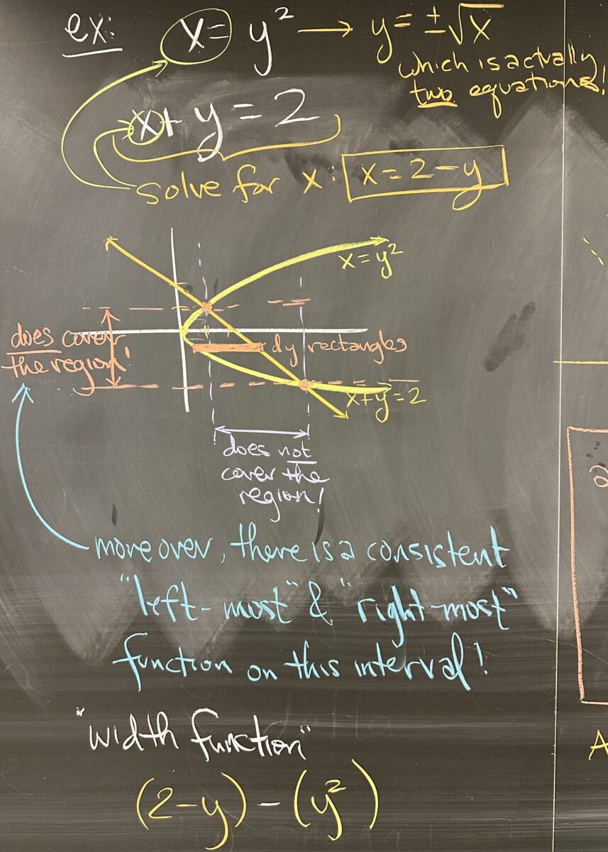
In the next example, we have two curves: \(x = y^2\) and \(x+y=2\). The first curve is explicitly given as \(x=f(y)\), so we should be thinking about using \(dy\) rectangles. If we attempt to rewrite this curve in the form \(y = f(x)\), we end up splitting the curve into two pieces: \(y = \sqrt{x}\) and \(y = -\sqrt{x}\). This is not a good situation, as we’d rather not make more equations to keep track of.
The second curve could go either way, solving \(x = 2-y\) or \(y = 2-x\). Our preference is to go with \(x=2-y\) because that matches the form from the first curve (and our \(dy\) strategy).
If we then graph the curves and consider the enclosed region, our intuition is confirmed when we see that the \(y\)-interval (from the intersection points) fully contain the enclosed region while the \(x\)-interval does not. This confirms that our strategy should be to use \(dy\) rectangles.
As with the quiz problem, we must then determine which curve is “greater”. By choosing \(y=0\) from our \(y\)-interval, we can see that \(x=2-y\) is greater than \(x=y^2\). As such, our width function is \((2-y) – (y^2)\).
If we finished this example, we would integrate our width function over the \(y\)-interval given by the intersections: \[\int_{-2}^1 -y^2-y+2\,dy\]
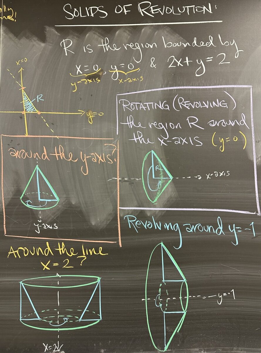
Expanding on the idea of regions bounded by curves, we move on to the topic of the day: Solids of Revolution. The core idea here is that we will take an enclosed region (like the ones we’ve been considering) and then rotate the region around a line, sweeping out a solid, 3-D shape.
Our example uses the region bounded by \(2x+y=2\), the \(x\)-axis, and the \(y\)-axis. The enclosed region is a right triangle, so then we consider several scenarios where this region is rotated around a line.
First, we look at what happens when the region is rotated around the \(x\)-axis. The \(x\)-axis is one of the boundaries of the region, so when we revolve the region, the result is a cone (whose “tip” sits at \(x=1\) on the \(x\)-axis). This cone has a base radius larger than its overall height, so the cone ends up being short and wide.
If we instead consider what happens when the region is rotated around the \(y\)-axis, the result is again a cone (whose “tip” sits at \(y=2\) on the \(y\)-axis). This cone has a larger height than its base radius, so the cone ends up being taller and more narrow than the \(x\)-axis revolution.
But what happens if we rotate the region around a line that doesn’t coincide with the boundary of the region?
If we rotate the region around the line \(y=-1\), we have a short and wide conical shape (as we saw rotating around \(y=0\), the \(x\)-axis). However, because of the gap between the axis of revolution (\(y=-1\)) and the region, there is a hollow cylinder along the center of the conical shape. The solid of revolution ends up being a cone with a cylindrical hole “drilled” through it from tip to base.
Alternatively, if we rotate the region around the line \(x=2\), the conical surface forms the inside of the solid rather than the outside. From the outside, our solid looks like a cylinder. Overall, we end up with a cylinder with a conical shape “carved” out of the center.
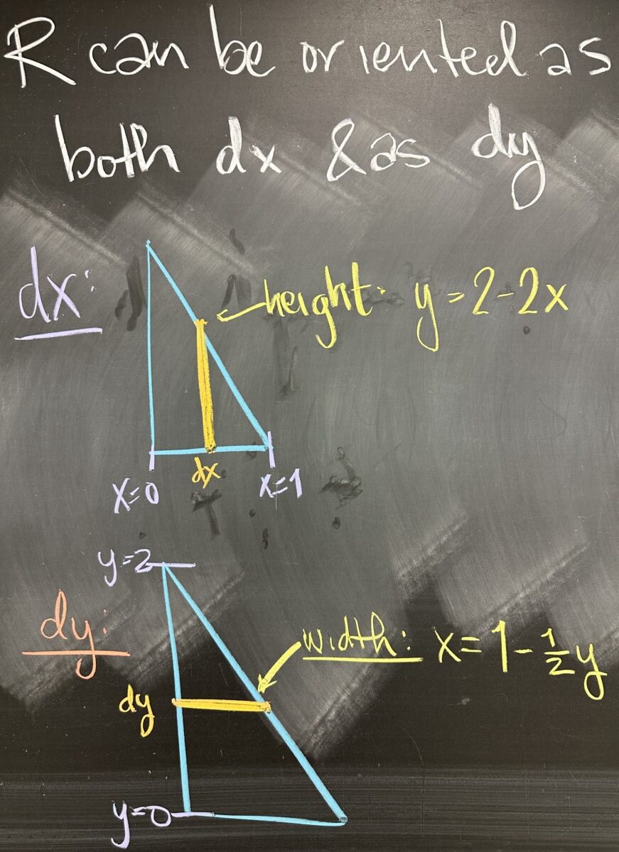
This particular region is flexible as the intersection points form intervals that fully enclose the region in both the \(x\)- and \(y\)-directions. This means we have the option of using either \(dx\) or \(dy\) rectangles. In the image, we see the region set up with \(dx\) rectangles (tall and narrow) over the interval \(0 \leq x \leq 1\), followed by an image of the region set up with \(dy\) rectangles (wide and short) over the interval \(0 \leq y \leq 2\).
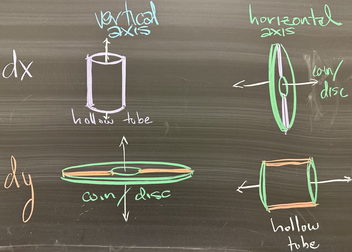
To wrap things up, we consider what happens when we rotate \(dx\) or \(dy\) rectangles around vertical or horizontal axes. There are four possible combinations, but there ends up being only two possible outcomes: either a hollow tube (thin walls — either \(dx\) or \(dy\) thickness) or a disc (flat, with thickness \(dx\) or \(dy\)).
After our exam on Tuesday, we’ll come back to this topic to go over how we will find the volumes for these two possible outcomes.


Recent Comments