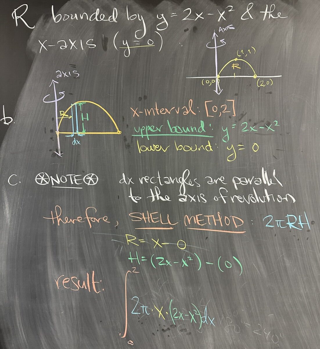
Today’s quiz covered the topic of Volumes of Solids of Revolution. Our region for the quiz is bounded by the equations \(y = 2x-x^2\) and \(y=0\) (the \(x\)-axis), and the axis of revolution is the line \(x=0\) (the \(y\)-axis). The first question asked for a sketch of the region along with labels for any intersections, which you can see in the image above.
The equation \(y=2x-x^2\) is a parabola that opens downwards, and through some quick factoring, we can find its intersections with the \(x\)-axis to be \((0,0)\) and \((2,0)\).
The next question on the quiz asked for an analysis of the region from the perspective of “dx” rectangles. This means that \(x\) will be our independent variable, and the interval for \(x\) will be \([0,2]\). We must also consider the height of our rectangles, measured in the \(y\)-direction (though \(x\) is our independent variable and we aim to express height in terms of \(x\)). Our upper bound for the region is \(y=2x-x^2\) and the lower bound is \(y=0\).
The third part asked for the method that is required for this region and axis of revolution when combined with “dx” rectangles. Since our rectangles are parallel to the axis of revolution, we should recognize that the situation calls for the “shell method”.
The shell method requires both \(R\), the radius (distance from the axis of revolution), and \(H\), the height of the rectangle. Again, we will want to express both in terms of \(x\), the independent variable. The axis of revolution is \(x=0\), so the radius will be \(R=x-0\). The height of our rectangles is given by the difference between the upper and lower bounds of our region: \(H=(2x-x^2)-0\).
Putting it all together, the integral for the volume is: \[\int_a^b 2\pi R H\,dx = \int_0^2 2\pi x \left(2x-x^2\right)\,dx\]
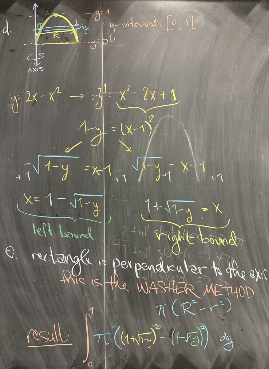
Moving on to the “dy” perspective, first note that our independent variable will be \(y\). This means that bounding curves must be written in terms of \(y\) (solved for \(x\)). Solving \(y=2x-x^2\) for \(x\) requires completing the square, \(1-y=x^2-2x+1=(x-1)^2\), followed by careful splitting using both positive and negative square-roots to end up with two equations: \(x=1-\sqrt{1-y}\) (the left boundary of our region) and \(x=1+\sqrt{1-y}\) (the right boundary).
With \(y\) as the independent variable, the interval for \(y\) is \([0,1]\), the smallest interval that encloses the entire region.
For the next part, since the “dy” rectangles are perpendicular to the axis of revolution, we should recognize that the situation calls for the “washer method”. In this case, we say “washer” instead of “disc” because our region is not bounded by the axis of revolution. Looking at our sketch, we can see that our rectangle is not bordering on the axis of revolution — and as a result, revolving the rectangle will result in a disc with a hole (a “washer”).
The washer method relies on two radii: one inner radius and one outer radius. The outer radius is the one farthest from the axis of revolution — in our case, that is \(x=1+\sqrt{1-y}\). The inner radius is the one closest to the axis of revolution: \(x=1-\sqrt{1-y}\).
Putting it all together, the integral for the volume is: \[\int_a^b \pi(R^2-r^2)\,dy = \int_0^1 \pi\left((1+\sqrt{1-y})^2-(1-\sqrt{1-y})^2\right)\,dy\]
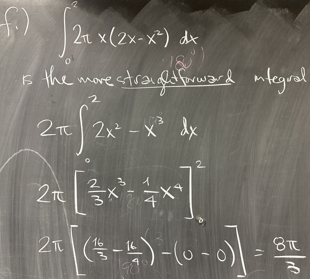
Of the two options for computing the volume, the first integral is by far the most straightforward. Now, in practice, it is not realistic to construct both integrals before deciding which one to work out. Judging by the original equation for our parabola, we should note that it is expressed as \(y=f(x)\) — solved for y — with \(x\) as the independent variable. This is a strong indicator that we should keep \(x\) as our independent variable by working with “dx” rectangles.
Indeed, we see that the “dx” setup works out to be the more straightforward of the two methods. Working out the integral, we factor out the coefficient of \(2\pi\), distribute multiplication by \(x\), then apply the power rule and evaluate the antiderivative at the bounds and subtract: \[2\pi\int_0^2 2x^2-x^3\,dx = 2\pi\left[\left(\frac{16}{3}-\frac{16}{4}\right)-\left(0-0\right)\right] = \frac{8\pi}{3}\]
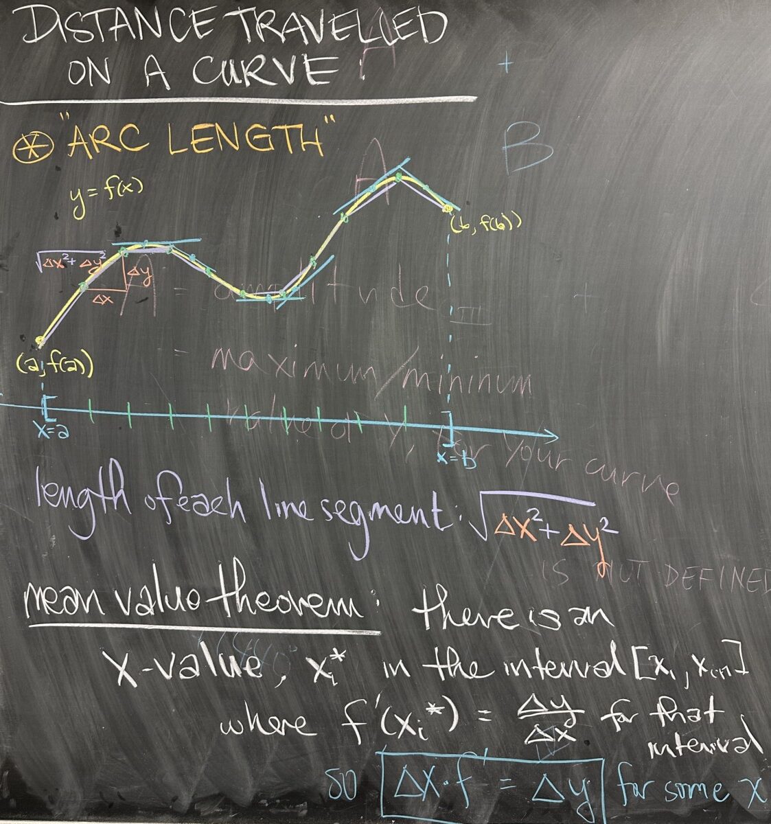
Today’s topic attempts to answer the question, “what is the length of a curve given by a function?” Length, or distance, is easily measured in straight lines, but quite a challenge along curves. When attempting to measure distance along a curve on an interval \([a,b]\), we can begin by dividing the interval into sub-intervals, just as we have done for Riemann Sums, or for Solids of Revolution.
Under this sub-interval approach, we get a collection of points on the curve, which we can connect them with straight lines (with easy distances to compute) to form an approximation of the curve. Each segment of this approximation is a straight line, with length \(\sqrt{\Delta x^2+\Delta y^2}\).
On each sub-interval, we can apply the Mean Value Theorem (which I hope you recall from Calculus I). The Mean Value Theorem (under certain conditions) guarantees that on each sub-interval we can find an \(x\)-value, \(x_i^*\), where the derivative has value equal to the slope between the endpoints of our interval: \(f'(x_i^*) = \frac{\Delta y}{\Delta x}\).
Considering that our approximation will ultimately be the subject of a limit as the number of sub-intervals grows to infinity, we should understand that our sub-intervals will eventually each collapse to a single point, and with an infinite number of them, they represent every point in the interval \([a,b]\). We can also consider this result from the Mean Value Theorem in terms of linear approximation and differentials: \(f'(x) \approx \frac{\Delta y}{\Delta x}\) which can be written equivalently: \(\Delta y \approx f'(x)\,\Delta x\), noting that they will achieve equality in the limit.
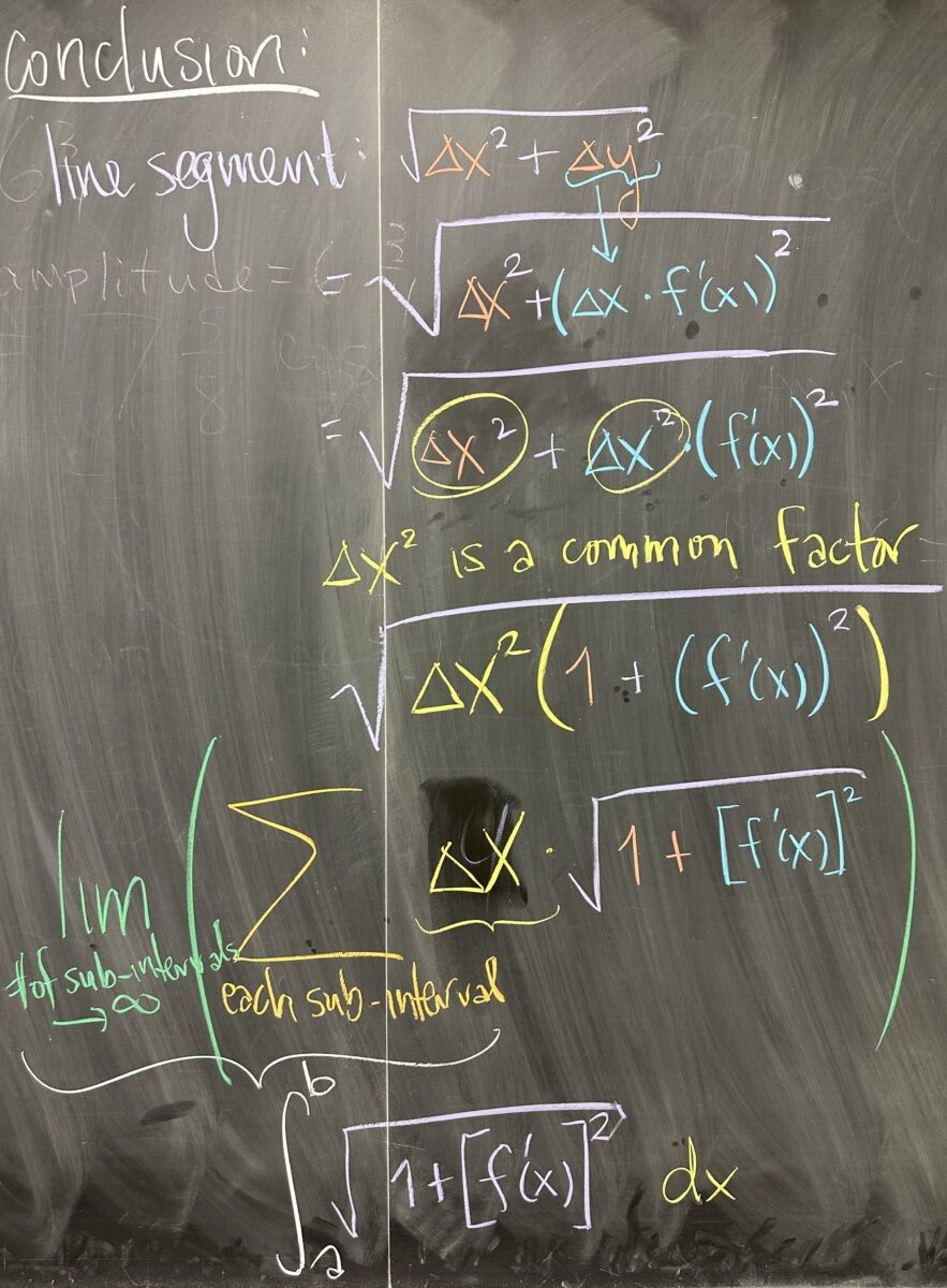
With the Mean Value Theorem in hand, we can replace \(\Delta y = f'(x)\,\Delta x\) in our length expression for each segment of our approximation: \[\sqrt{\Delta x^2 + \Delta y^2} = \sqrt{\Delta x^2 + \left(f'(x)\cdot \Delta x\right)^2}\]
From here, we can factor out \(\Delta x^2\) from the radicand: \[\sqrt{\Delta x^2 + \left(f'(x)\right)^2 \cdot \Delta x^2} = \sqrt{\Delta x^2 \left(1 + \left(f'(x)\right)^2\right)}\]
Distributing the \(\frac{1}{2}\) exponent across the product (and simplifying \(\sqrt{\Delta x^2} = \Delta x\)): \[\sqrt{\Delta x^2 \left(1 + \left(f'(x)\right)^2\right)} = \Delta x \sqrt{1+\left(f'(x)\right)^2}\]
This has all been the simplification of the computation of length for a single line segment. As for the approximation of the entire length of the curve, we consider the sum of \(\sqrt{1+\left(f'(x)\right)^2} \Delta x\) over all the sub-intervals. Furthermore, we know that all of this is happening in the limit as the number of sub-intervals grows to infinity.
The limit of sums over an interval, \([a,b]\), follows our original framework for definite integrals: \[L = \int_a^b \sqrt{1+\left(f'(x)\right)^2} \, dx\]
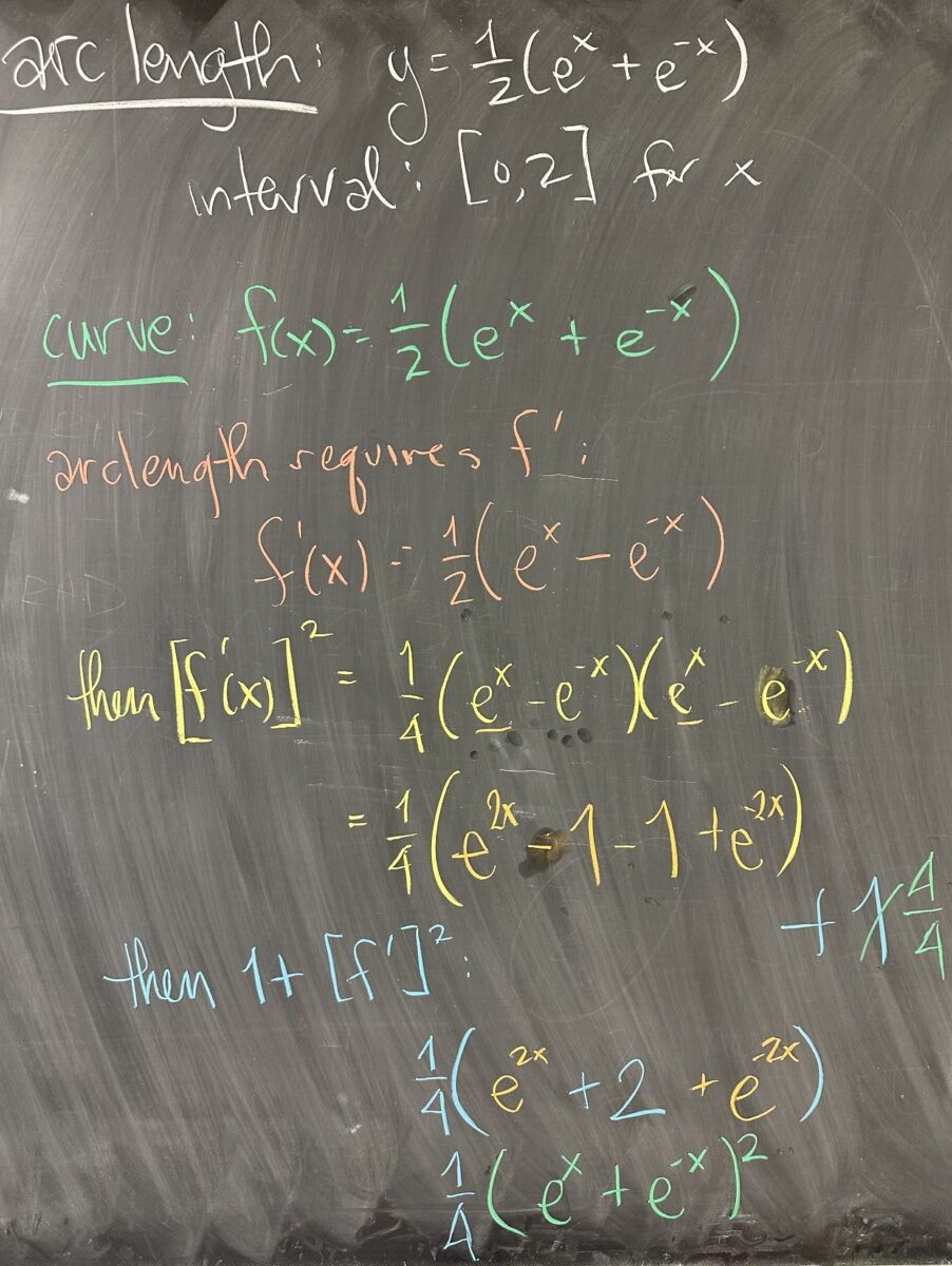
If we attempt to find the arc length of the curve \(y = \frac{1}{2}\left(e^x+e^{-x}\right)\) over the \(x\)-interval \([0,2]\), the derivative of our curve is necessary for the integrand: \(\sqrt{1+\left(f'(x)\right)^2}\).
Starting with \[f'(x) = \frac{1}{2}\left(e^x+e^{-x}\cdot -1\right) = \frac{1}{2}\left(e^x-e^{-x}\right)\]
Then squaring the result: \[\left(f'(x)\right)^2 = \left(\frac{1}{2}\left(e^x-e^{-x}\right)\right)^2 = \frac{1}{4}\left(e^{2x}-2+e^{-2x}\right)\]
Adding one: \[\left(f'(x)\right)^2+1 = \frac{1}{4}e^{2x}-\frac{1}{2}+\frac{1}{4}e^{-2x} + 1 = \frac{1}{4}e^{2x}+\frac{1}{2}+\frac{1}{4}e^{-2x}\]
Note that this result is a perfect square: \[\left(f'(x)\right)^2+1 = \frac{1}{4}\left(e^{2x}+2+e^{-2x}\right) = \frac{1}{4}\left(e^x+e^{-x}\right)^2\]
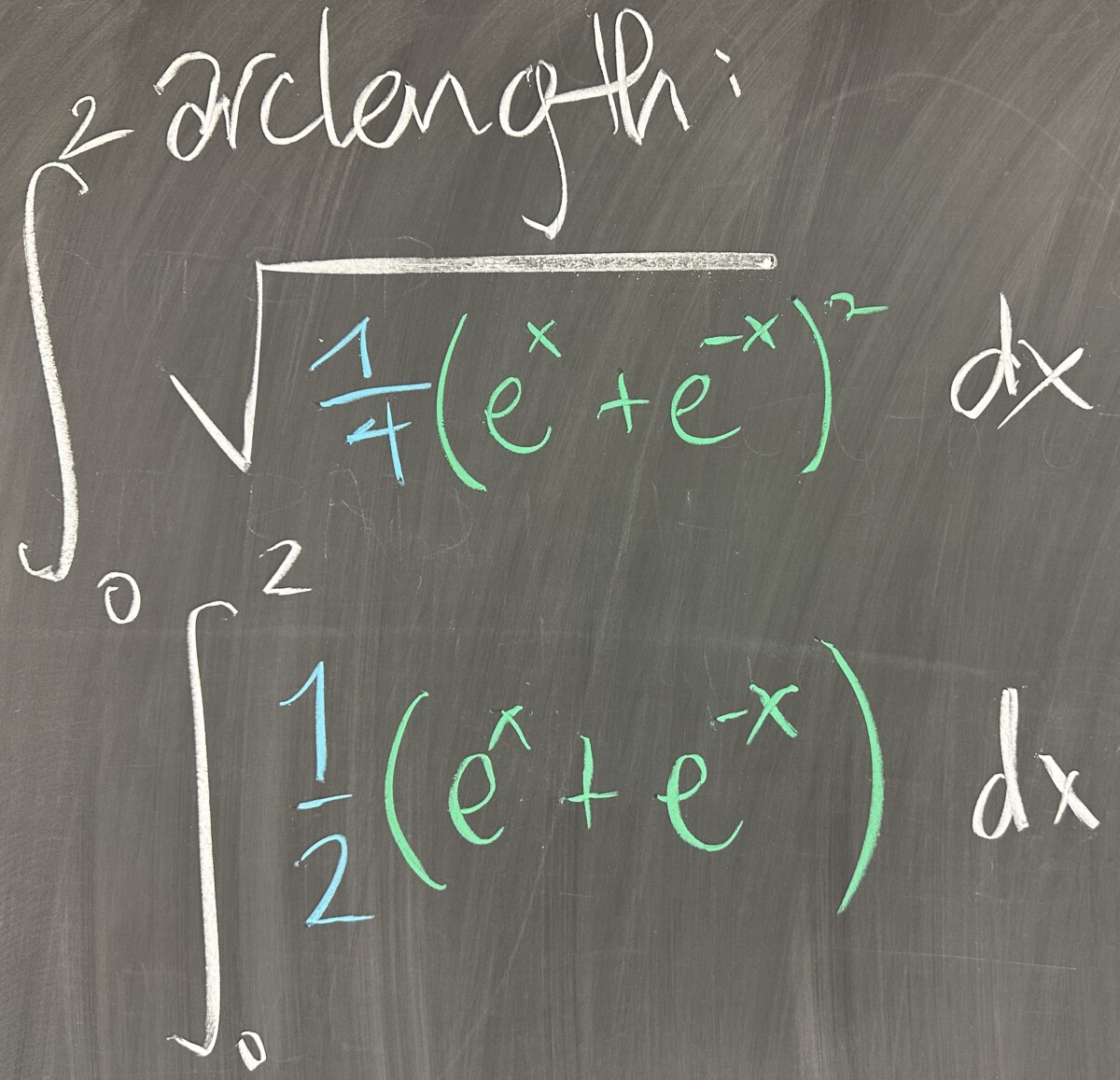
Then the square root of \(1+\left(f'(x)\right)^2\): \[\sqrt{1+\left(f'(x)\right)^2} = \sqrt{\frac{1}{4}\left(e^x+e^{-x}\right)^2} = \frac{1}{2}\left(e^x+e^{-x}\right)\]
So our arc length integral is \[\int_a^b \sqrt{1+\left(f'(x)\right)^2}\,dx = \int_0^2 \frac{1}{2}\left(e^x+e^{-x}\right)\,dx\]
Finishing the computation, noting that \(\int e^x\,dx = e^x\) and \(\int e^{-x}\,dx = -e^{-x}\): \[\int_0^2 \frac{1}{2}\left(e^x+e^{-x}\right)\,dx = \frac{1}{2}\left(e^x-e^{-x}\right)\Bigg\vert_0^2 = \left(\frac{e^2}{2}-\frac{1}{2e^2}\right)-0\]


Recent Comments