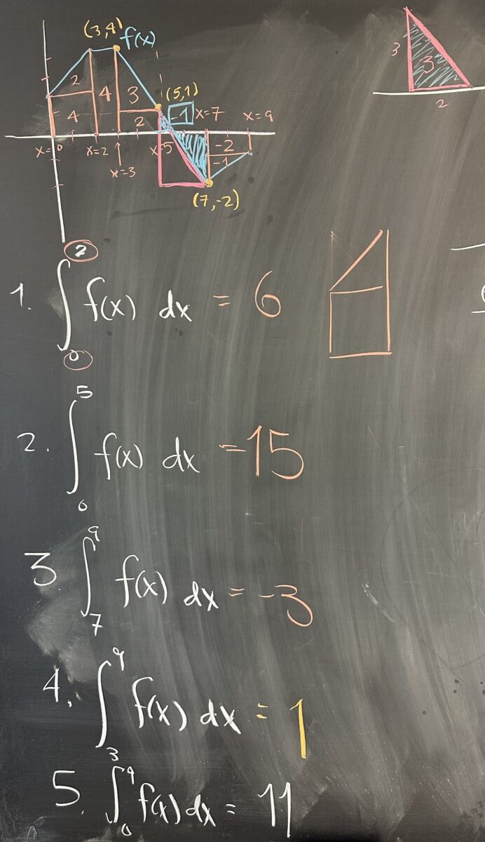
Today’s quiz focused on the interpretation of our notation: \(\displaystyle\int_a^b f(x)\, dx\). This notation refers to the area between \(f(x)\) and the \(x\)-axis, from \(x=a\) to \(x=b\).
Given the graph of \(f(x)\), we can determine this area using rectangles and triangles.
The trickiest of these computations was #4
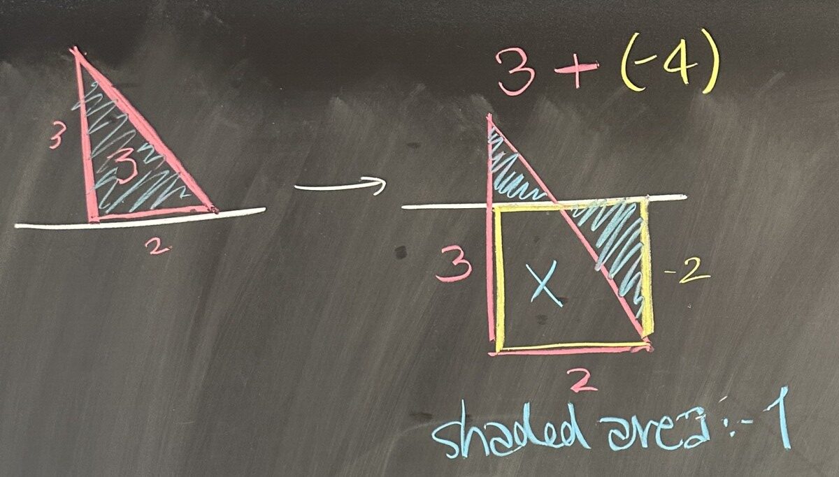
If we consider the triangle as sitting directly on the \(x\)-axis, and then consider the difference between that and where the \(x\)-axis actually sits (relative to the triangle). The triangle has total area of \(3\) square units, and the yellow square has area \(4\) square units. Subtracting the square from our triangle, we end up covering the blue shaded area, counted positively for the smaller upper triangle, and counted negatively for the larger, right-most triangle.
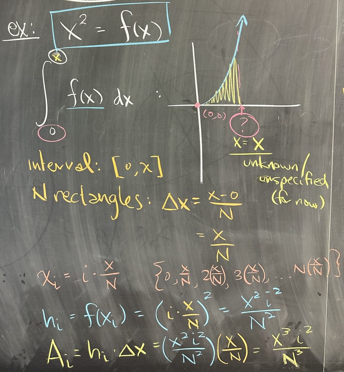
For today’s lesson, we start by picking up a modified version of the problem we left off with on Tuesday. We attempted to determine the the area bounded by our function (\(f(x) = x^2\)) and the \(x\)-axis, starting at \(x=0\) up to an unspecified \(x\)-value.
We divide our interval \([0,x]\) into \(N\) rectangles, determine our \(x\)-values (\(x_i\)), and then we use those to compute our heights (\(h_i\)) and then our areas (\(A_i\)).
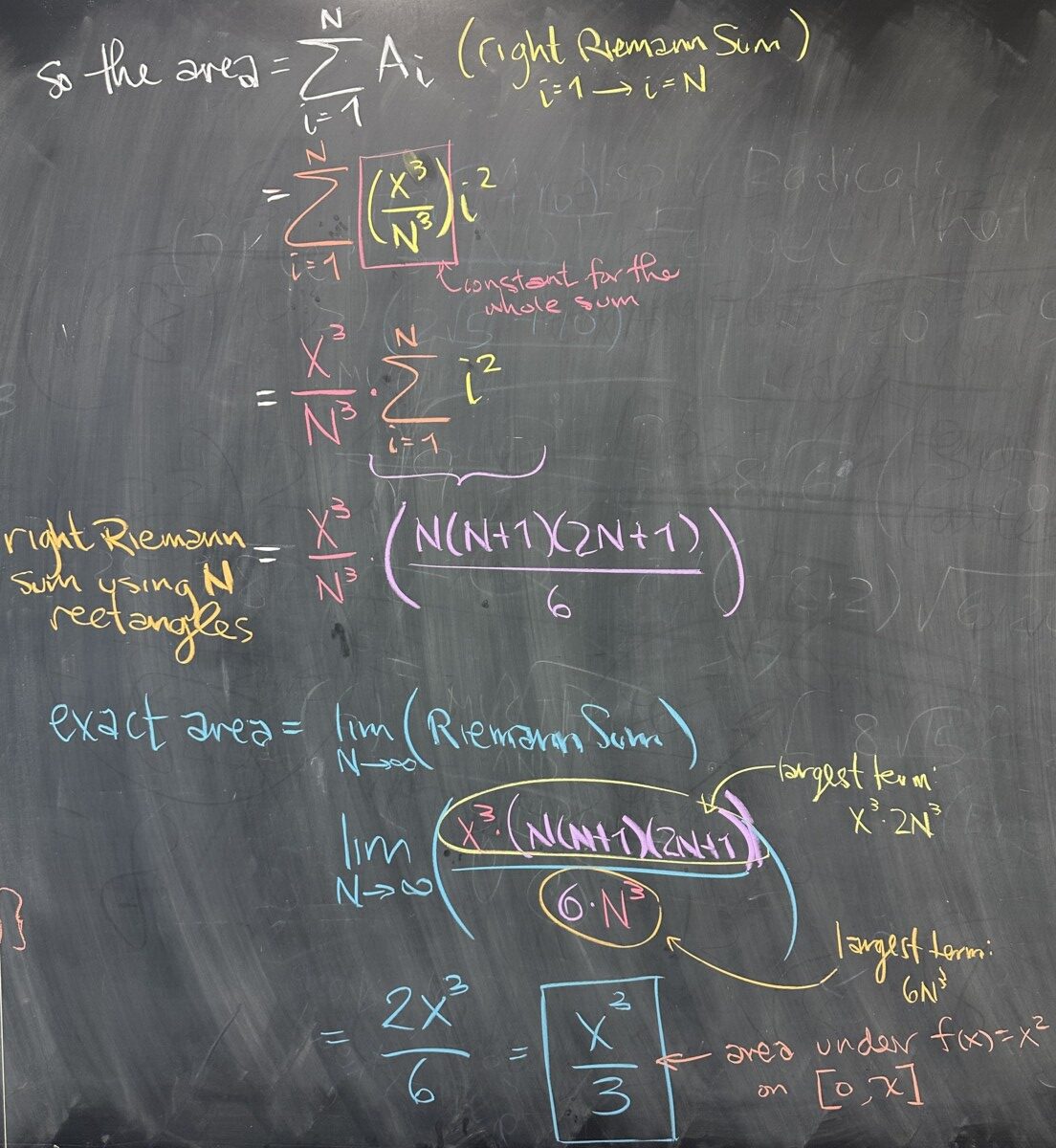
Once we have our areas, \(A_i\), we take the sum to represent the total area. This is a finite sum over the rectangles starting with \(i=1\) (the first rectangle) to \(i=N\). In this sum, \(i\) is changing, but \(x\) and \(N\) are not. Because of this, we should recognize that \(\frac{x^3}{N^3}\) will remain constant as \(i\) increments through the values from \(1\) to \(N\). As a result, we can factor \(\frac{x^3}{N^3}\) from the sum. The result is \(\displaystyle\frac{x^3}{N^3}\sum^\infty_{i=1} i^2\), and we know a closed form for \[\sum^\infty_{i=1} i^2 = \frac{N(N+1)(2N+1)}{6}\] \[\frac{x^3}{N^3}\sum^\infty_{i=1} i^2 = \frac{x^3}{N^3}\frac{N(N+1)(2N+1)}{6}\]
With our formula for the (right) Riemann Sum in hand, we can take the limit as \(N\to\infty\) to get the exact area.
We find that the degree of our numerator and denominator are equal, so the limit exists and is given by the ratio of the coefficients of the highest degree terms: \(\frac{2x^3}{6} = \frac{x^3}{3}\).
This might not seem all that interesting, but what we found is that \[\int_0^x x^2\, dx = \frac{x^3}{3}\]
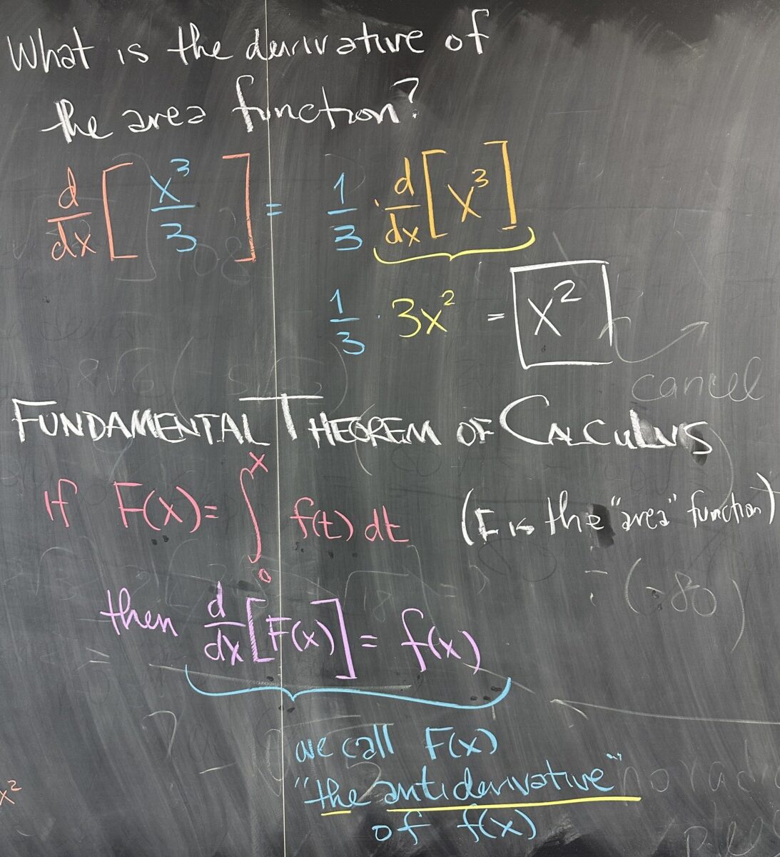
The interesting thing about our result is that the derivative of our area function \(\frac{x^3}{3}\) is equivalent to our original \(f(x) = x^2\). This is no fluke, it is actually true for all functions. This relationship is so important that it has a name:
“The Fundamental Theorem of Calculus”.
The Fundamental Theorem of Calculus is usually described as having two parts. Which part is ‘first’ and which is ‘second’ varies depending on your source. In our lesson, the first part is the relationship we just discovered from \(\int_0^x x^2\,dx = \frac{x^3}{3}\).
First part: “the derivative of the area (function) bounded by \(f(x)\) on the interval \([0,x]\) is equivalent to the original function, \(f(x)\)”.
We define the area function as \(\displaystyle F(x) = \int_0^x f(t)\,dt\), using \(t\) to avoid repeated use of \(x\) for different purposes. This “area function”, \(F(x)\) is referred to as an “antiderivative” of the original \(f(x)\). Note that \(f\) is the derivative of \(F\), making \(F\) the “antiderivative” of \(f\).
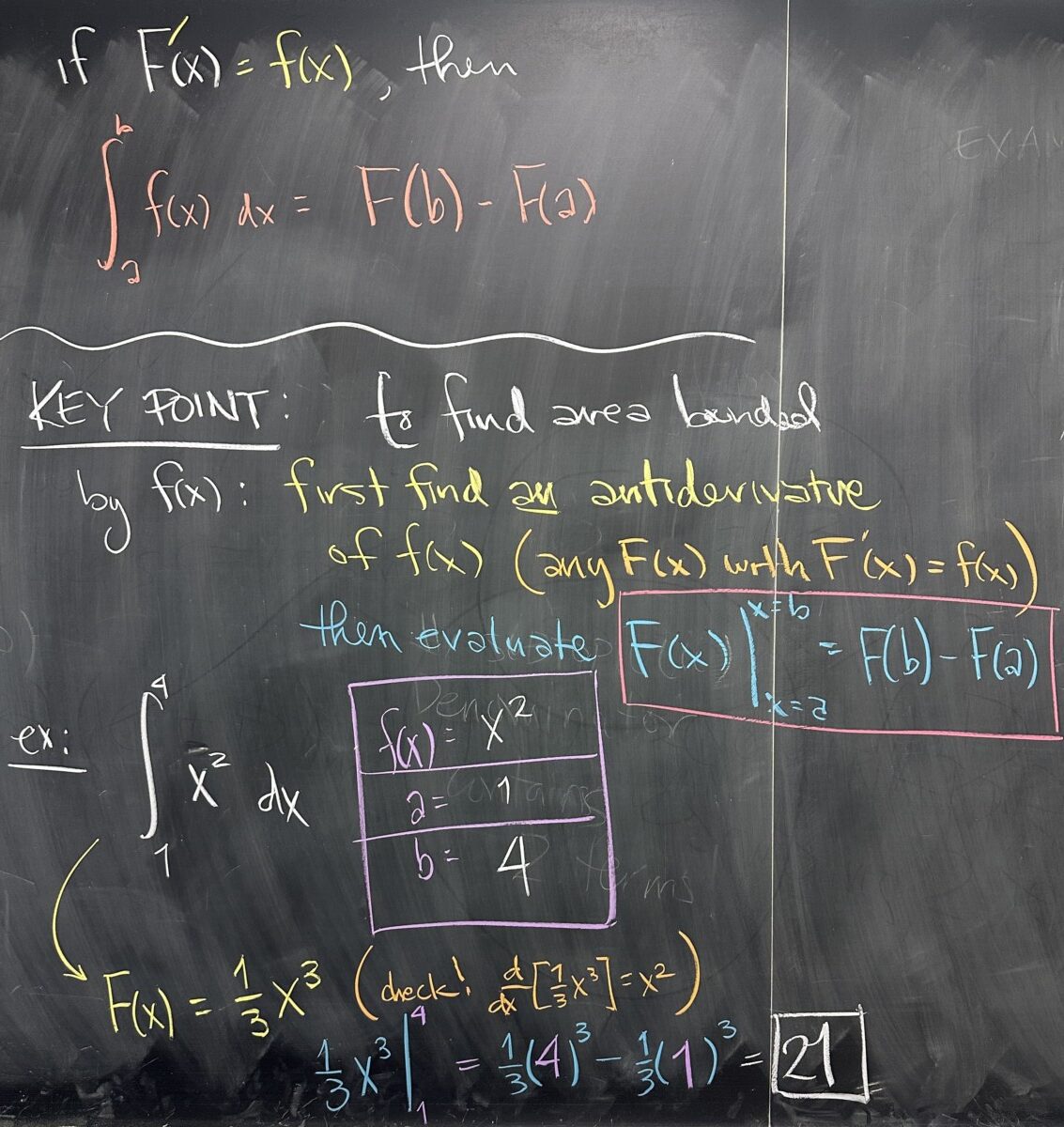
The second part (for us): if we have (any) antiderivative of \(f(x)\), in other words some \(F(x)\) with derivative \(F'(x) = f(x)\), then the area bounded by \(f(x)\) and the \(x\)-axis is given by the antiderivative. \[\int_a^b f(x)\,dx = F(b) – F(a)\]
Our key takeaway here is that antiderivatives hold the key to finding the area bounded by functions.
- First, find an antiderivative of the function that bounds the area we want to find.
- Then evaluate the antiderivative at \(x=b\) and \(x=a\) and subtract.
We looked at a quick example using the same function (whose antiderivative we already found): \[\int_1^4 x^2\,dx = \frac{1}{3}x^3\left.\right\vert_1^4 = \frac{1}{3}4^3 – \frac{1}{3}1^3 = 21\]
Because our calculations for area will require antiderivatives, it is crucial that we all focus on understanding functions and their derivatives — with an emphasis on thinking about reversing the derivative process.
Our first task is thinking about how to find an antiderivative for a polynomial term, \(x^n\). Since the power rule determines the process for taking the derivative of such terms, we seek to reverse it.
Power rule on \(x^n\) — finding the derivative:
- multiply by the exponent, \(n\), as a coefficient
- reduce the exponent by one, to \(n-1\)
- \(\displaystyle\frac{d}{dx}\left[x^n\right] = n x^{n-1}\)
Reversing this process on \(x^n\) — finding the antiderivative:
- increase the exponent by one, to \(n+1\)
- divide by the exponent, \(\frac{1}{n+1}\) as a coefficient
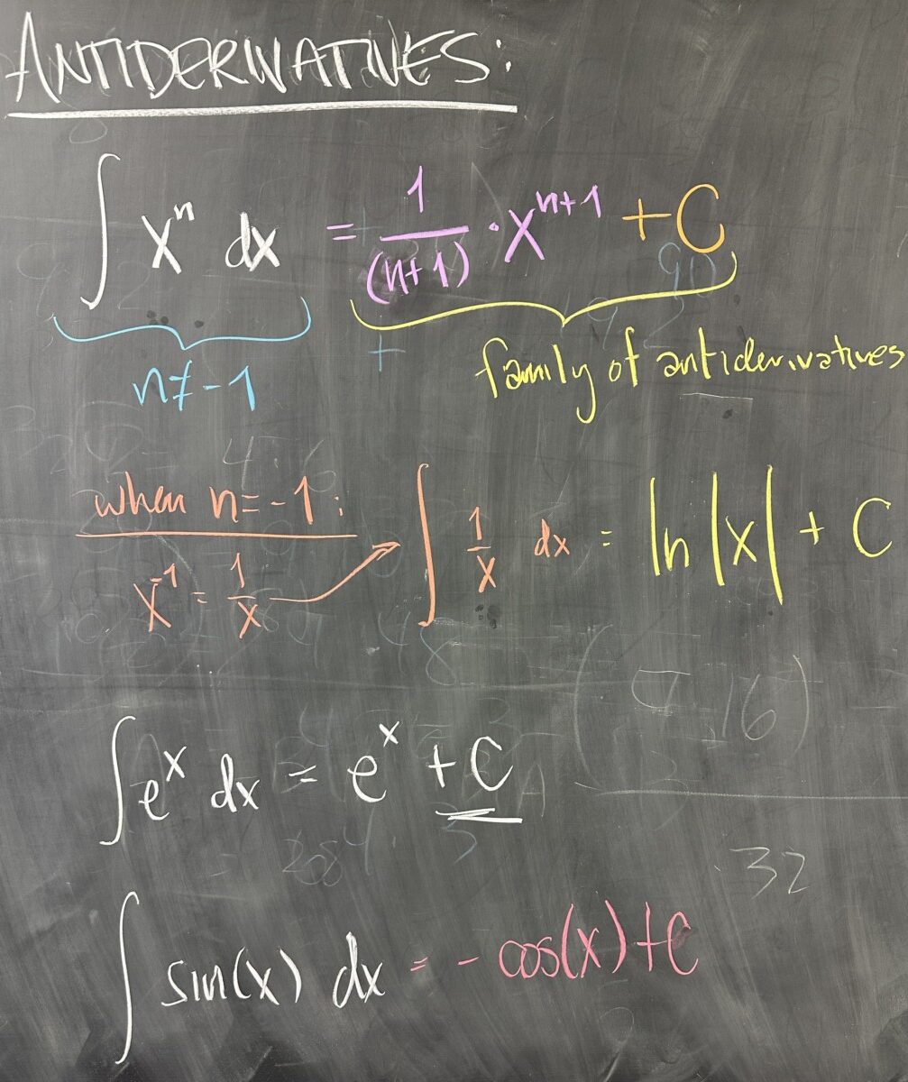
- \(\displaystyle\int x^n\,dx = \frac{1}{n+1}x^{n+1} + C\)
You will note that our antiderivative includes \(+C\), where we consider “C” as an unspecified constant value. This is because the derivative of any constant is zero: \(\frac{d}{dx}[C] = 0\).
Put in another way, the antiderivative, as a function, can be shifted vertically without affecting the slope of the tangent line (a.k.a. the derivative). So we have not only one antiderivative for a given \(f(x)\), we actually have an entire “family” of antiderivative functions.


Recent Comments