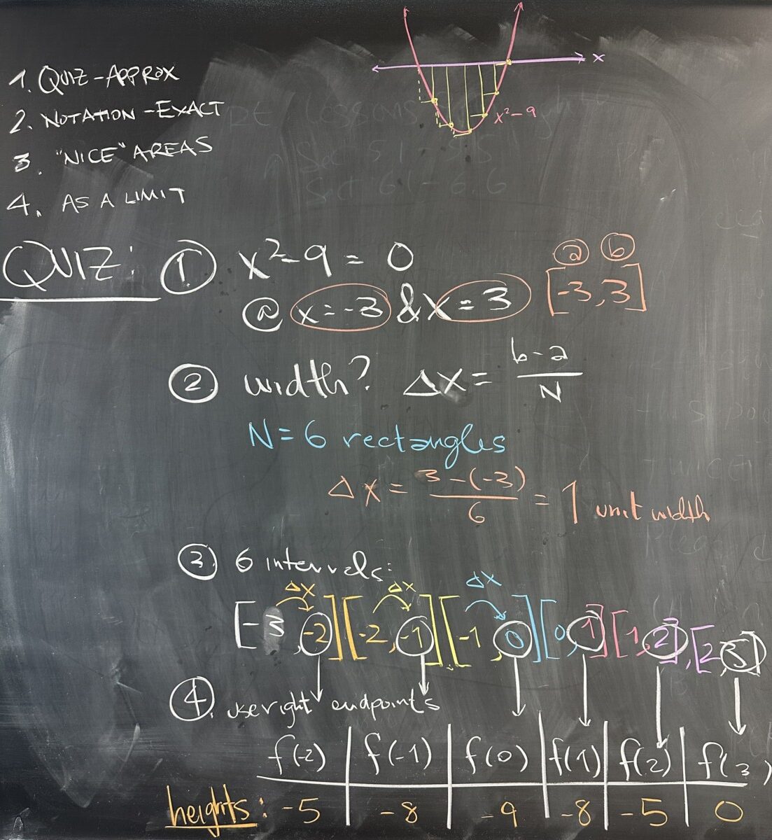
Today’s quiz covered the Riemann Sum. The given function was \(f(x) = x^2 – 9\), and you were asked to identify where the function intersected the \(x\)-axis. These two intersections were then used as the start and end of our interval for approximating the area bounded by \(f(x)\).
The different questions on the quiz were arranged to walk you through the necessary steps to find the Riemann Sum. First we identified the width of each rectangle based on the fact that we were told to use \(N = 6\) rectangles. So, \(\Delta x = \frac{3-(-3)}{6} = 1\). From there, we established the six individual intervals for each rectangle — where the width of each rectangle is \(\Delta x = 1\).
The next quiz question asked you to find the area of each rectangle \(A = H \times W\), and we know \(W = \Delta x \ 1\). So we must find the missing \(H\) for each rectangle. The quiz instructed you to use the right endpoint of each interval, so we take that \(x\)-value and plug it into \(f(x)\) to get a \(y\)-value which we can use for \(H\).
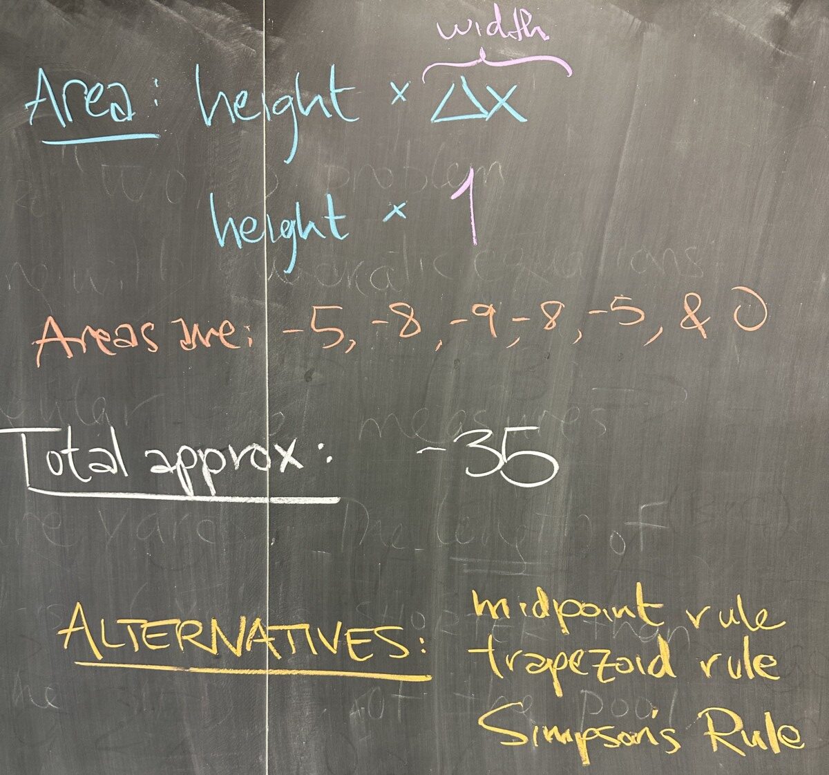
Once we have the area of each rectangle (remember, there should be \(N = 6\) areas, one for each rectangle), we take the sum to find the total approximated area.
There are many improvements on the Riemann Sum approximation, which we did not have time to discuss. I listed a few in case you want to look into them.
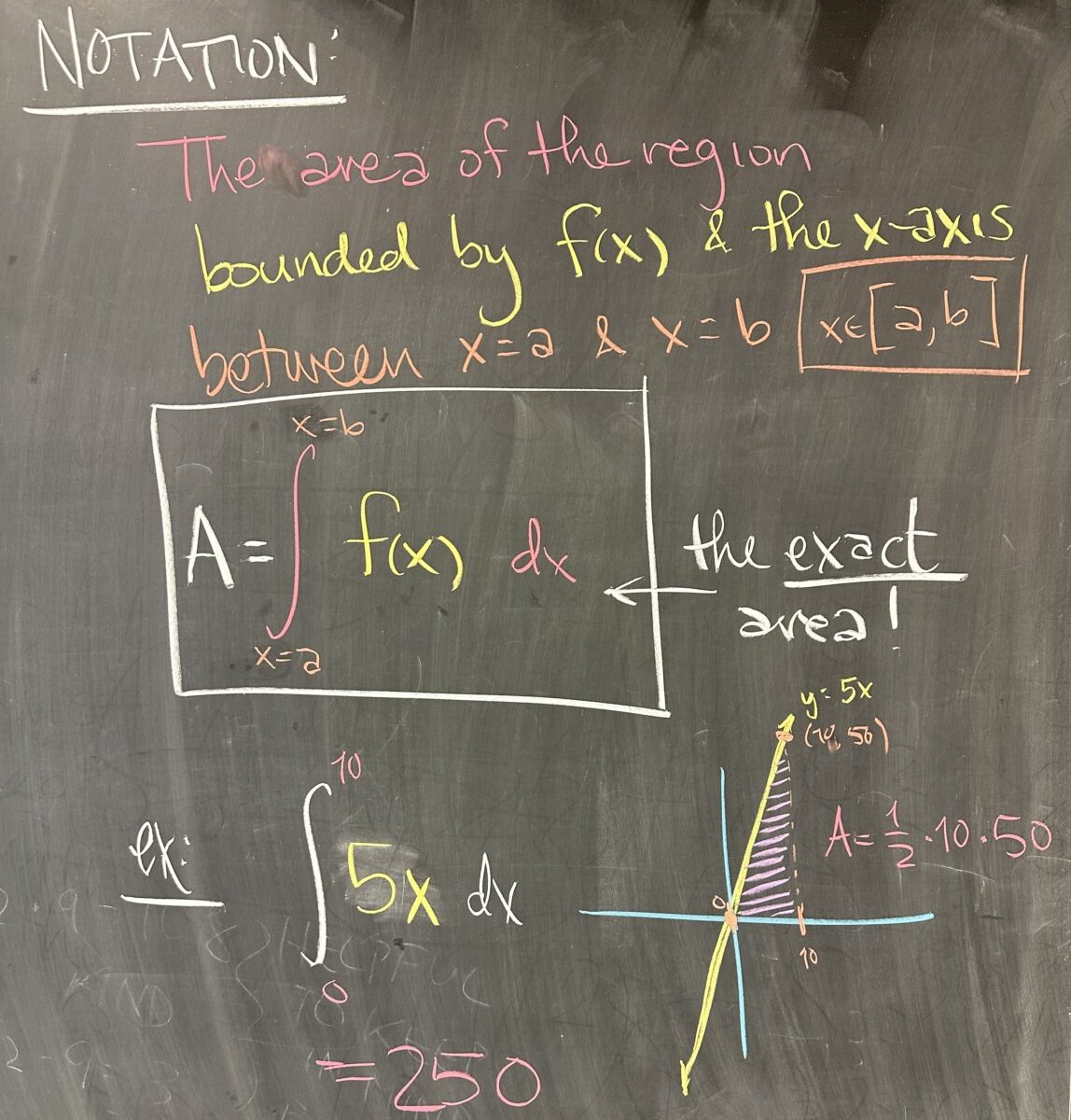
Moving on to new material, we started out with the notation for the areas that we have been trying to approximate. This notation is used to describe the exact area enclosed by a function and the \(x\)-axis (between \(x = a\) and \(x = b\)).
Our first example ended up giving us the shape of a right triangle, whose area is easy to compute \( A_{\triangle} = \frac{1}{2}WH\). In this case, our \(W = 10\) and our \(H = 50\), so \(A = 250\). Using our new notation: \[\int^{10}_0 5x\, dx = 250\]
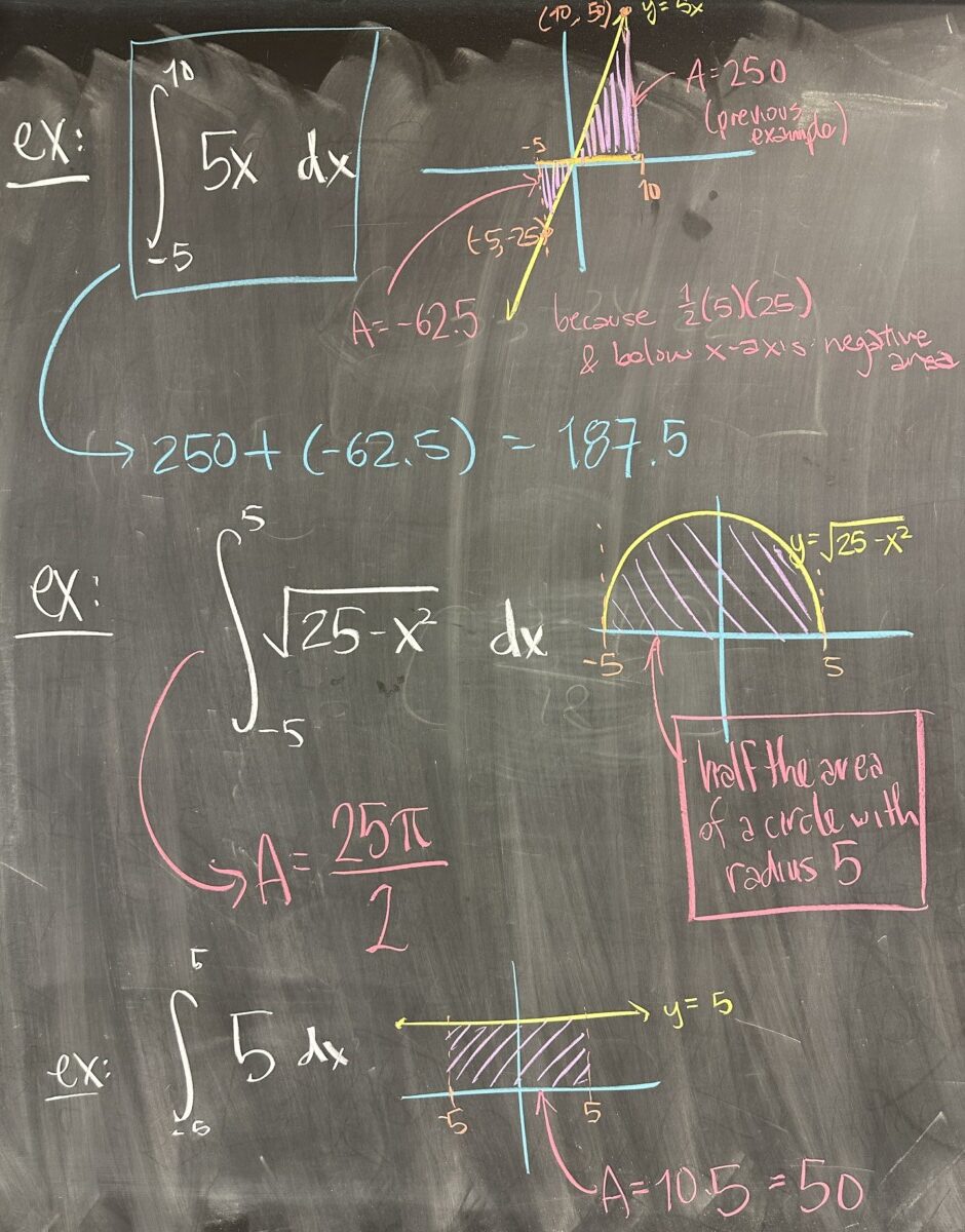
The next example is an expansion of the previous one, where we consider an interval for \(x\) that includes \(x\)-values for which our function will be negative (thus creating ‘negative area’). Here we consider the entire enclosed region as two separate triangles, and find the total area by adding their individual areas together.
The third example is that of a semi-circle. \(f(x) = \sqrt{25 – x^2}\) is the upper-half of the circle (centered at the origin) with radius: 5. The region enclosed by \(f(x)\) and the \(x\)-axis between \(x=-5\) and \(x=5\) is exactly half of the circle with radius 5. So the area is half that of the circle, or \(A = \frac{1}{2} \pi 5^2\).
The last example on this slide is the area bounded by the horizontal line \(f(x) = 5\), the \(x\)-axis, and the vertical lines \(x=-5\) and \(x=5\). This region is a simple rectangle, and the area is just \(A = 10 \times 5\).
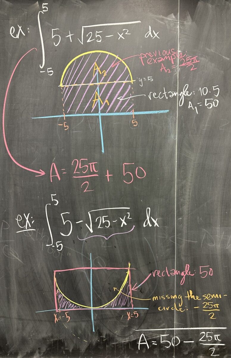
The next two examples attempt to show what happens when we combine functions: \(f(x) = 5\) and \(g(x) = \sqrt{25-x^2}\).
First, \(f(x) + g(x)\). In this case, we see the semi-circle shifted up by 5 units. This effectively creates the same area as the original semi-circle, but now with the area of the rectangle from the previous slide underneath it. The total area is just the sum of the semi-circle (from \(g(x)\)) and the rectangle (from \(f(x)\)).
In the second, we have \(f(x) – g(x)\), which gives us the bottom half of the semi-circle (again) shifted up by 5 units. The resulting enclosed region is effectively the rectangle from the previous slide without the semi-circle. So in calculating the area of the enclosed region, we use the area of the rectangle minus the area of the semi-circle.
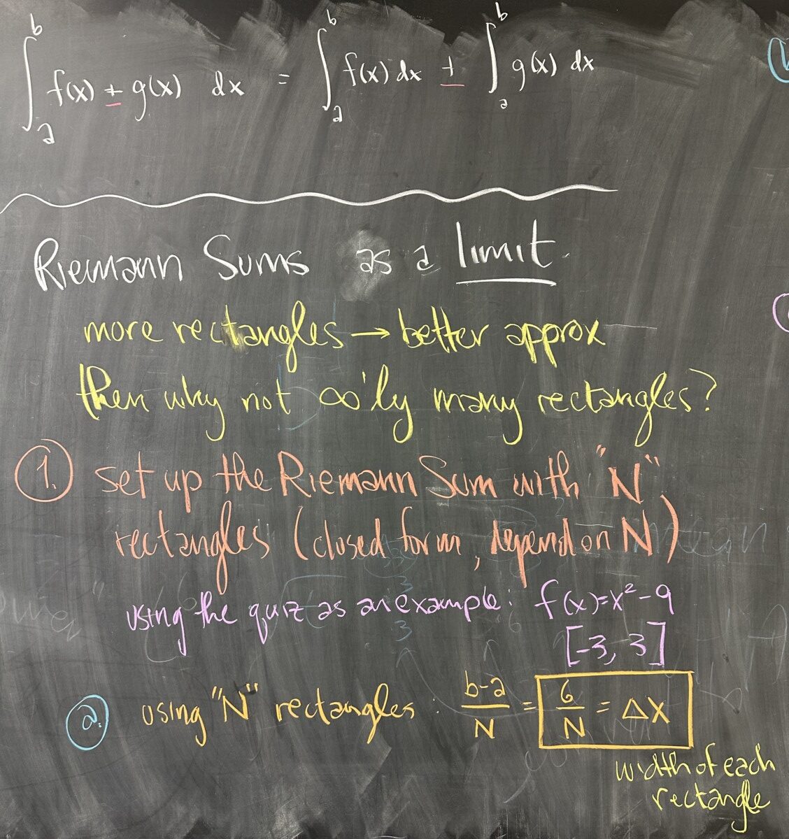
We then formalize the relationship of areas computed from combinations of functions as follows: \[\int_a^b \left(f(x) + g(x)\right)\, dx = \int_a^b f(x) \, dx + \int_a^b g(x) \, dx\]
At the end of the lesson, we turned our attention back to the Riemann Sum approximation and attempted to use it to find the exact area. If the use of more rectangles causes the Riemann Sum to be a better approximation, then we could find the Riemann Sum as a function of \(N\), the number of rectangles, and then take the limit as \(N \to \infty\).
Our first step is to compute the Riemann Sum without specifying the number of rectangles — so \(N = N\), unspecified. This means our \(\Delta x = \frac{6}{N}\), and it’s okay! We expect that \(N\) appears many places in our calculations.
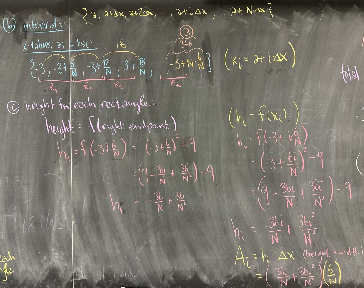
We then start listing the endpoints of our rectangle-intervals by repeatedly adding \(\Delta x\), one at a time. This is the process of an arithmetic sequence (starting with \(i = 0\)), \[x_i = a + i \cdot \Delta x = -3 + i \cdot \frac{6}{N} \]
To compute the height of each rectangle, recall that we must plug \(x\)-values into our function to get \(y\)-values (which we can use as height, since \(y\) is measured vertically). We did the first right endpoint as an example, but then it is going to be too much work (not to mention we don’t have a specific \(N\) number of rectangles) to do this for each \(x\)-value separately.
Instead, we use the established pattern for the \(x_i\) and plug that into our function to get a pattern for the heights: \[h_i = y_i = f(x_i) = \left(-3 + \frac{6i}{N}\right)^2 – 9\]
After some algebra (FOIL the squared binomial), we end up with \(h_i = -\frac{36i}{N} + \frac{36i^2}{N^2}\).
Once we have the height of each rectangle, \(h_i\), we can then find the area of each rectangle, \(A_i\), by multiplying height by width — recalling that width is \(\Delta x = \frac{6}{N}\). \[A_i = h_i \cdot \Delta x = \left(-\frac{36i}{N} + \frac{36i^2}{N^2}\right)\left(\frac{6}{N}\right)\] \[A_i = -\frac{216i}{N^2} + \frac{216i^2}{N^3} \]
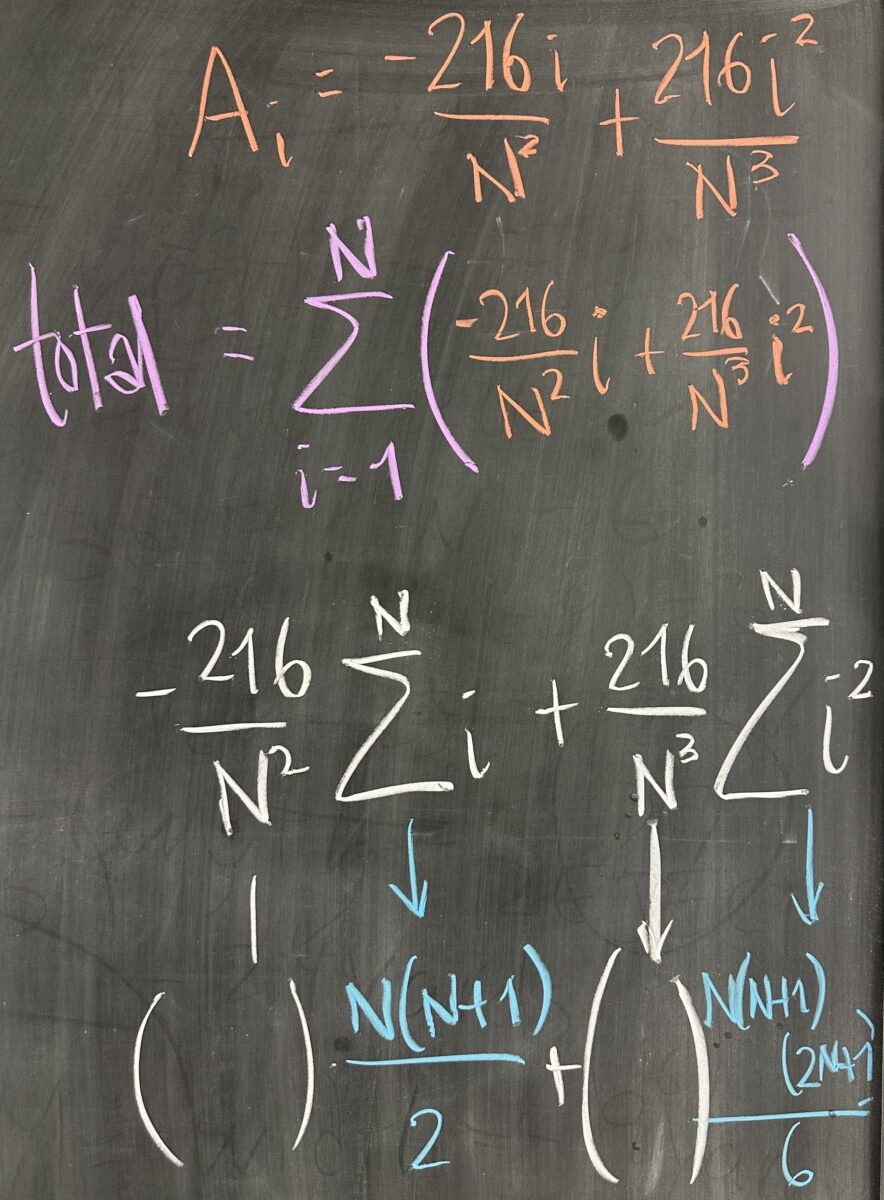
Once we have the areas for each rectangle, \(A_i\), we must add the areas to get a total: \(\displaystyle\sum^N_{i=1} A_i\) \[\sum^N_{i=1} \left(-\frac{216i}{N^2} + \frac{216i^2}{N^3}\right)\]
Now, this sum indicates that \(i\) is changing values, starting at \(i = 1\) and ending at \(i = N\). It is important to recognize that \(N\) is not changing in this sum. We did not choose a specific value for \(N\), but \(N\) itself does not change when computing the total area. As a result, we can treat \(N\) as constant — and to be clear, \(i\) is not constant. With this in mind, we can rearrange the sum as follows: \[\sum^N_{i=1} \left(-\frac{216i}{N^2} + \frac{216i^2}{N^3}\right) = \sum^N_{i=1} -\frac{216}{N^2}i + \sum^N_{i=1} \frac{216}{N^3}i^2\]
where: \[\sum^N_{i=1} -\frac{216}{N^2}i = -\frac{216}{N^2} \sum^N_{i=1} i\]
and: \[\sum^N_{i=1} \frac{216}{N^3}i^2 = \frac{216}{N^3} \sum^N_{i=1} i^2\]
From the previous unit on sums/series, we know that the finite sum of \(i\) from \(1\) to \(N\) is equal to \(\frac{N(N+1)}{2}\); and we also know that the finite sum of \(i^2\) from \(i=1\) to \(i=N\) is equal to \(\frac{N(N+1)(2N+1)}{6}\).
As a result, we can simplify: \[-\frac{216}{N^2} \sum^N_{i=1} i = -\frac{216}{N^2} \cdot\frac{N(N+1)}{2}\]
and: \[\frac{216}{N^3} \sum^N_{i=1} i^2 = \frac{216}{N^3} \cdot \frac{N(N+1)(2N+1)}{6}\]
Remember that the total area was the sum of these two expressions, so the Right Riemann Sum for \(f(x) = x^2 – 9\) from \(x=-3\) to \(x=3\) using \(N\) rectangles is: \[R_N = -\frac{216}{N^2} \cdot\frac{N(N+1)}{2} + \frac{216}{N^3} \cdot \frac{N(N+1)(2N+1)}{6}\]
Which we can simplify: \[ R_N = -\frac{108N(N+1)}{N^2} + \frac{36N(N+1)(2N+1)}{N^3}\]
At home, see what happens if you now use \(N = 6\) — you should get the same result as we did at the beginning of this lesson. The quiz used this same function, with the same bounds, and \(N = 6\). We should get the same approximate area both ways.
We did not have time to complete this in class, but look at our expression for \(R_N\). \(R_N\) is the sum of two rational functions, each with the same degree in the numerator and denominator. This means \(R_N\) has a horizontal asymptote, which further tells us that the \(\displaystyle\lim_{N\to\infty} R_N\) will be a real number. This limit gives us the exact area for the region. Please compute this limit and be prepared to give it as a bonus answer on Thursday’s quiz.


Recent Comments