
Contents
Patterns of Inheritance: Fruit Flies, Blood Types, Population Genetics and Hardy-Weinberg
Lab Overview
Over the next four weeks we will be working with two different exercises and simulations to further examine patterns of inheritance. In the first series of labs you will perform monohybrid and dihybrid crosses using real fruit flies (Drosophila melanogaster) to examine inheritance patterns. The labs are spread out over a course of four weeks due to the time it takes to cross and rear flies. The second set of labs deals with inheritance patterns of human blood types. During the “down time” of the fly lab, you are expected to work on the blood typing activity and become familiar with the genetics behind different blood types. You are also expected to become familiar with the Hardy-Weinberg principle, and how it can be used as a null model to determine if evolution has occurred in a population. Finally, you will perform computer simulations of population genetic processes during Week 6.
Lab Breakdown
Week 4 – Examination of wild-type and mutant Drosophila phenotypes and sex identification. Begin blood typing exercise.
Week 5 – F1 phenotyping, setting up F1 crosses. Continue working on blood typing exercise.
Week 6 – Remove all adult F1 flies from cross vials. Perform population genetic simulations.
Week 7 – Score phenotypes of all F2 flies. Data analysis and review.
Drosophila Genetics
The fruit fly, Drosophila melanogaster, is a ‘model organism’ that has been used for genetics research for many years. These flies have a relatively short generation time, are easy to cross, produce a large number of offspring, have relatively small genomes, and are harmless to humans, making them an ideal study system to understand patterns of inheritance in a controlled laboratory setting. We will be studying inheritance patterns of both wild-type and mutant phenotypes of flies over the course of several weeks. In Week 5 you will cross F1 flies exhibiting different phenotypic characteristics. Crosses may be either monohybrid or dihybrid. You goal will be to determine which traits are dominant, recessive, autosomal, and sex-linked. To help guide you through the activities it will be useful to think back to what you learned about Mendelian inheritance and Punnett squares.
Fly Lab Week 4 – Sexing Fruit Flies and Quantifying Phenotypes
For the first portion of the fruit fly exercise your goal is to become familiar with determining the sex of flies. Although this can be difficult at times, there are a few key criteria that can be used to help make the determination. Male flies generally have a darker posterior region versus females, whereas the female abdomen tends to show several distinct stripes (Fig. 1).
.")
In addition to determining the sex of your flies (with a stereomicroscope or magnifying glass), you are expected to become familiar with the different phenotypes present in mutant and wild-type varieties. Pay particular attention to eye color and wing shape. Your instructor will provide anesthetized flies and petri dishes for your analysis. Fill in the table below with your observations and make sketches of the phenotypes and the sexes. When finished, transfer your flies to the vial of alcohol.
Table 1. Phenotypes of wild-type and mutant parental strains.
| Phenotype | Phenotype |
| Wild Type: | Mutant A: |
| Wild Type: | Mutant B: |
| Wild Type: | Mutant C: |
Space for sketches:
Fly Lab Week 5 – Quantification of F1 Phenotypes and Setting Crosses
This week you will be scoring F1 phenotypes and setting up F1 crosses to produce the F2 generation. F1 flies were already produced for you by crossing two pure strains together (from Table 1 above). Before you make your crosses, fill out the table below with your observations for F1 flies from particular parental strains (P generation).
Table 2. Sex-specific phenotypes of F1 flies.
____________________ X _____________________
Female Parent (P gen) Male Parent (P gen)
| Date | Phenotype | # Females With Phenotype | # Males With Phenotype | Total Number of Flies |
The next step is to setup your F1 crosses. As a class, we need to make sure that all crosses are made in replicate to obtain a decent sample size.
1. To setup your culture vials, add one cup of the Instant Drosophila Medium and 15 mL of water to the vial. When the solution solidifies, add 4-7 grains of yeast to the culture media.
2. Add six (6) male/female pairs of anesthetized flies into your culture vial. Be sure to label the vial with ‘F1 cross’, the parental strains crossed, the date, and your names.
3. After all the F1 flies are scored, the data are recorded, and the crosses set, dispose of any remaining anesthetized F1 flies into the vial with alcohol.
4. Based on the data in Tables 1 and 2, come up with a hypothesis for how your trait(s) are inherited. For example, how many genes are involved? Which alleles are likely dominant and recessive? Are any traits sex-linked?
5. Create two Punnett squares showing the results of both your P and F1 crosses. You may use any letters you like for alleles. Results will vary depending on which strains your group selected for crosses.
6. What are the predicted phenotypic ratios of your F2 generation?
Fly Lab Week 6 – Removing F1 Flies from Crossing Vials
The fly activities this week are relatively short. Thus, this is a good time to focus on the population genetics simulation lab and the associated questions and the end of the manual. At this point in the experiment you will need to remove the F1 flies from your crossing vials. This is necessary to prevent mating between F1 and F2 flies, which will bias the results. Also, by Week 6 you should begin to see F2 fly larvae emerging in your vials. Place your culture vial under a dissecting microscope to get a better look at the morphological features of your larvae. If possible, make some sketches of your larvae using the space below. Make sure your flies don’t escape!
1. Obtain an empty culture vial and plug.
2. Tap your F1 cross vial on your bench to knock the adult flies to the bottom. Remove plug and place mouth of empty vial on mouth of cross vial. Invert vials to transfer adult flies into the new vial. Quickly replace plug in both vials.
3. Anesthetize adult flies by dipping wand into Fly Nap anesthetic and inserting wand beside the plug.
4. When adequately anesthetized, place flies in alcohol vial.
Sketches of Larvae
Fly Lab Week 7 – Quantification of F2 Phenotypes and Data Analysis
Your goal this week is to score the phenotypes of the F2 flies that originated from your F1 crosses. Determine both the sex of each fly and the relevant phenotype(s). Anesthetize the adults and transfer them to a petri dish for scoring. Use the dissecting microscope or magnifying glass to aid in data collection. Try to score as many flies as possible and fill out the table below.
Table 3. Sex and phenotypic data for F2 offspring.
____________________ X _____________________
Female Parent (P gen) Male Parent (P gen)
| Phenotype (and sex) | Total |
Total scored _______________
Next, fill out the corresponding tables with class totals for each cross. Results will vary depending on which crosses were performed.
Table 4. F2 sex and phenotypic data for the entire class.
____________________ X _____________________
Female Parent (P gen) Male Parent (P gen)
| Phenotype (and sex) | Total |
Total scored _______________
___________________ X _____________________
Female Parent (P gen) Male Parent (P gen)
| Phenotype (and sex) | Total |
Total scored _______________
____________________ X _____________________
Female Parent (P gen) Male Parent (P gen)
| Phenotype (and sex) | Total |
Total scored _______________
- Calculate the observed phenotypic ratios for the class data for each cross.
____________________ X _____________________
Female Parent (P gen) Male Parent (P gen)
F2 phenotypic ratio:
____________________ X _____________________
Female Parent (P gen) Male Parent (P gen)
F2 phenotypic ratio:
____________________ X _____________________
Female Parent (P gen) Male Parent (P gen)
F2 phenotypic ratio:
2. Do the observed ratios correspond to the ratios you predicted? Discuss your reasoning.
3. Using the total observed class data for each cross, conduct chi-square analyses to determine if there is a statistically significant difference between observed and expected phenotypes. Remember, in a monohybrid cross we expect a 3:1 phenotypic ratio in the F2 generation, whereas in a dihybrid cross we expect a 9:3:3:1 ratio. Recall the chi-square formula:
^2}{E}=\frac{(O_1-E_1)^2}{E_1}+\frac{(O_2-E_2)^2}{E_2}")
The degrees of freedom (df) = # different F2 phenotypes – 1. Thus, df = 1 for a monohybrid cross and df = 3 for a dihybrid cross. Use the chi-square table to determine if your calculated chi-square values are statistically significant.

As an example, suppose you performed a monohybrid cross of wild-type and sepia-eyed flies and scored 100 F2 flies. Out of the 100 flies, 65 had the wild-type phenotype and 35 had the mutant (sepia) phenotype. Are the results significantly different from expectations (i.e. 3:1 ratio)?
^2}{E}=\frac{(65-75)^2}{75}+\frac{(35-25)^2}{25} = 1.33 + 4 = 5.33")
With 1 df and P = 0.05, a chi-square value of 5.33 is significantly higher than that expected by chance. Thus, we can conclude that the observed results are significantly different from expectations (i.e. we reject the null hypothesis of no statistically significant difference between observed and expected values).
Go ahead and perform your own series of calculations for each of the three crosses examined in class. Are any results consistent with expectations? Explain.
Human Blood Types
Human blood can be of four primary types: Type A, Type B, Type AB, and Type O. These types are determined based on a specific antigen present on an individual’s red blood cells. For example, someone with Type A blood possesses Type A antigen on red blood cells whereas someone with Type B blood has Type B antigen on his/her red blood cells (Fig. 1). Individuals with Type AB blood show a phenotype expressing both Type A and Type B antigens. Finally, someone with Type O blood has neither Type A or Type B antigens on red blood cells. In addition, individuals with certain blood types will possess antibodies in their blood that will react with different blood types. This is why doctors make sure that they know your specific blood type before a transfusion is given! For example, a normal individual with Type A blood will possess antibodies against Type B blood. If this individual was given a transfusion of Type B blood, the anti-B antibodies in the patient’s blood will bind the Type B antigen on the transfused blood, leading to agglutination, or the clumping of red blood cells. This can lead to reduced efficiency of oxygen transport in the body and death. Since individuals with AB blood have both Type A and Type B antigens, no antibodies to either are present in the blood. This is why blood type AB is considered the ‘universal recipient.’ They can receive blood from pretty much anyone without fear of a negative reaction. Conversely, people with Type O blood possess antibodies against both Type A and Type B. Thus, these individuals can only receive blood from others with Type O. However, since Type O blood cells do not contain any A or B antigen, any blood group can receive Type O blood. This is why blood type O is considered the ‘universal donor.’ Figure 2 provides a summary of donor and recipient status for different blood types. In addition to the ABO system, you will often see a + or – sign after the blood type. This designated whether the blood is positive or negative for a second antigen called a Rhesus or Rh-factor that is controlled by different genes.
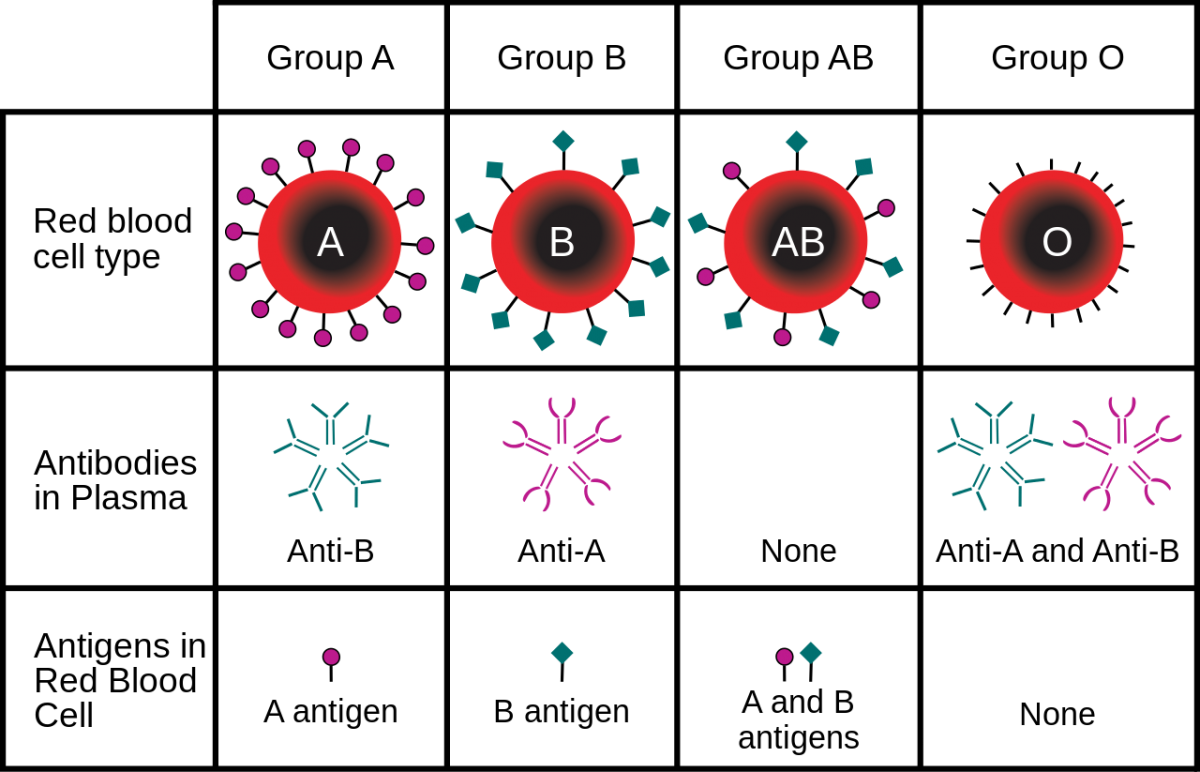
. twintiger007.")
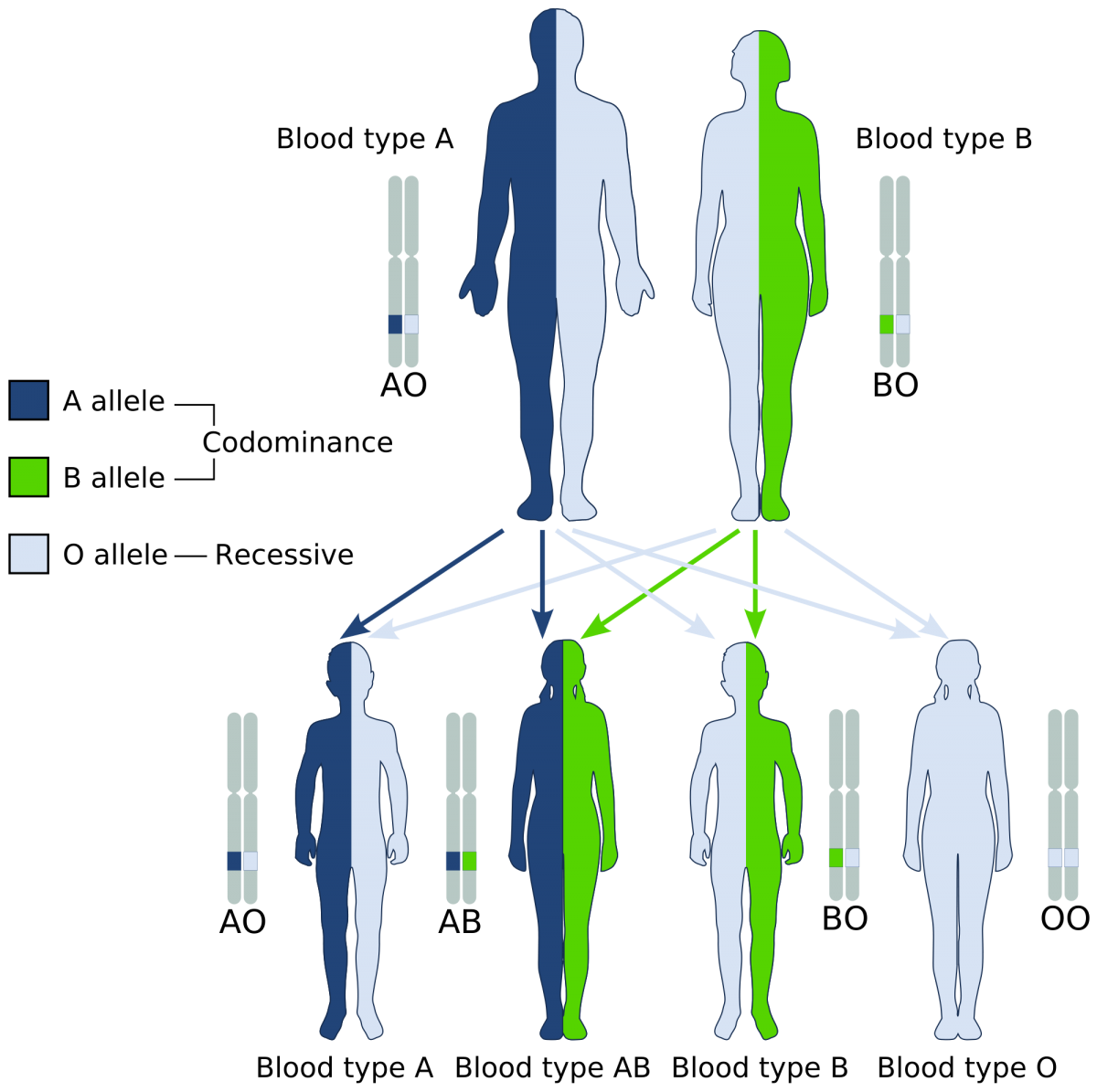
Inheritance of human blood type deviates from simple Mendelian assumptions. The first deviation is that three different alleles control the blood phenotype in the ABO system. These alleles are commonly designated IA, IB, and i. The A and B alleles are codominant, meaning that both phenotypes are expressed in heterozygotes (Fig. 3). The i allele is recessive, meaning that individuals with Type O blood must have two copies to demonstrate the O phenotype.
Using the allelic nomenclature above, Table 1 shows all of the potential genotypes and phenotypes in this system.
Table 1. Possible genotypes and corresponding phenotypes in the human ABO blood group.
| Genotype | Phenotype |
| IA IA | A |
| IA i | A |
| IB IB | B |
| IB i | B |
| IA IB | AB |
| i i | O |
Use a Punnett square to conduct a cross between a heterozygous male with a IA IB genotype with a heterozygous female with a IB i genotype. What are the resulting phenotypic ratios?
The Hardy-Weinberg principle is a null model in population genetics that is used to determine if evolution has occurred in a population. If all of the Hardy-Weinberg assumptions are met, we can conclude that the population is not evolving. In reality, populations are always evolving due to one or multiple microevolutionary forces that change allele frequencies from generation to generation. Remember, evolution is defined as changes in allele frequencies over multiple generations. Microevolutionary forces include the following:
1. Mutation – the spontaneous creation of a new allele in a population
2. Gene flow – the transfer of alleles from one population to another
3. Natural selection – the influence of the environment on relative fitness of individuals in a population. Some alleles in a population might be selected for, whereas others will be selected against.
4. Genetic drift – changes in allele frequencies due to mating efficiency and randomness associated with allelic segregation during gametogenesis and meiosis (Fig. 4).
5. Nonrandom mating – sometimes considered a microevolutionary force due to changes in genotype frequencies.
.")
Let’s explore the Hardy-Weinberg (HW) principle in more detail. Suppose we are studying a gene in a population that consists of two alleles, we will call A and a. I tell you that the A allele is dominant and the a allele is recessive. Using HW notation, we call the A allele p and the a allele q. You also know that the frequency of p is 0.73.
What is the frequency of q?
p + q = 1
q = 1 – p
q = 1 – 0.73 = 0.27
Next, we can predict the genotype frequencies in the population under the HW assumption. Because we are generally working with diploid individuals possessing two alleles per gene/locus, we can come up with a formula to estimate genotype frequencies from allele frequencies.
(p + q)(p + q) = p2 + 2pq + q2 = 1
where p2 is the genotype frequency for the homozygote dominant genotype, 2pq is the genotype frequency of heterozygotes, and q2 is the genotype frequency for the homozygote recessive.
Using the allele frequencies of A and a above, calculate the genotype frequencies expected under HW assumptions.
As stated above, the HW principle is used as a null model to determine if a population is evolving. In practice, researchers collect genotypic data from a population of interest and compare the real genotypic data from the expected values under HW. Significant deviations from HW assumptions suggest that one or more microevolutionary forces are changing allele and genotype frequencies over generations.
Let’s try an example. Say you go out to a tropical island to study the population genetics of a species of lizard. For one of the genes you are examining you find only two alleles in the population, we will call T and t. You use molecular genetic tools to obtain the following genotypes for 100 lizards:
TT = 44
Tt = 36
tt = 20
Are these data consistent with HW expectations? Explain your reasoning and show your work. Raise your hand if you need assistance! Hint: calculate p first!
As with earlier problems, we can use a chi-square test to statistically test if the observed data differ from HW expectations. For HW tests with two alleles we use 1 degree of freedom because once we know p, q can be easily determined and vice versa. In the chi-square table the critical value at P = 0.05 is 3.84. Thus, calculated chi-square values > 3.84 suggest that the population is deviating significantly from HW expectations.
^2}{E}=\frac{(O_1-E_1)^2}{E_1}+\frac{(O_2-E_2)^2}{E_2}+\frac{(O_3-E_3)^2}{E_3}")
Blood Type Activity (Weeks 4 – 5)
As stated above, we will be working with this lab for two weeks along with the fruit fly and simulation labs. Your goal is to use synthetic blood samples to determine blood genotypes of an island population of humans with unknown ancestry. Some island inhabitants suggest that they share ancestry with populations on a neighboring island, whereas others suggest that the majority of their genetic makeup comes from foreign populations. We will be performing multiple rounds of blood testing over the course of two weeks, keeping track of the total number of counts for each blood type. The blood dishes can be reused, but make sure you rinse them well before testing different samples. The mixing sticks may be thrown away after use. However, be sure to use the correct color stick depending upon the treatment (blue, yellow, clear).
- Obtain a mixing tray and a blood sample from your instructor. Place a drop of blood into each of the three wells in your dish. Be sure to replace cap on sample.
- Add drop of Anti A (blue vial) in well labeled ‘A.’
- Add drop of Anti B (yellow vial) in well labeled ‘B.’
- Add drop of Anti D (clear vial) in well labeled ‘Rh.’
- Use the appropriately colored mixing stick to mix the blood sample with the serum. Make sure not to contaminate your samples! Dispose of mixing sticks when finished.
- Monitor wells to determine if agglutination occurs (this should hopefully be obvious). Fill in the table below with a ‘yes’ or ‘no’ depending on whether or not agglutination occurred. A positive reaction will indicate the blood type (e.g. a ‘yes’ for Anti-A only would signify an A- blood type). Each student will test two samples each week.
Week 4 data
| Sample # | Sample # | |
| Anti-A | ||
| Anti-B | ||
| Anti-Rh | ||
| Blood type |
Week 5 data
| Sample # | Sample # | |
| Anti-A | ||
| Anti-B | ||
| Anti-Rh | ||
| Blood type |
- Each week we will make a class tally of the different blood types. Fill in each table below.
Week 4 data (Island 1)
| Blood Group | Totals for Group | Blood Group Frequency |
| A+ | ||
| A- | ||
| B+ | ||
| B- | ||
| AB+ | ||
| AB- | ||
| O+ | ||
| O- |
Week 5 data (Island 2)
| Blood Group | Totals for Group | Blood Group Frequency |
| A+ | ||
| A- | ||
| B+ | ||
| B- | ||
| AB+ | ||
| AB- | ||
| O+ | ||
| O- |
- For each week, use the total class data to calculate the HW expected genotype frequencies for alleles controlling Rh factor. Assume that there are two alleles we will call D and d. Individuals with a DD or Dd genotype show the Rh+ phenotype and dd individuals are Rh-. Hint: calculate q2 and q first!
- The tables below shows the blood group frequencies of inhabitants of two different islands neighboring the islands that you have already scored above. What can you conclude based on these blood group frequencies and the genetic makeup of all islands?
Island 3
| Blood Group | Blood Group Frequency |
| A+ | 0.31 |
| A- | 0.05 |
| B+ | 0.01 |
| B- | 0.01 |
| AB+ | 0.01 |
| AB- | 0.01 |
| O+ | 0.43 |
| O- | 0.17 |
Island 4
| Blood Group | Blood Group Frequency |
| A+ | 0.07 |
| A- | 0.22 |
| B+ | 0.1 |
| B- | 0.1 |
| AB+ | 0.08 |
| AB- | 0.2 |
| O+ | 0.08 |
| O- | 0.15 |
- For the two additional island populations in Question 9, calculate the expected Rh factor genotype frequencies under HW equilibrium. How do the results compare to the two populations you blood typed? Explain your reasoning.
- So far, we have only examined HW principles in genes consisting of two alleles. We can extend the HW equations to more than two alleles, although the math can get confusing quickly. However, it isn’t much more difficult to calculate expected frequencies with three alleles. Our blood type activity provides an excellent example as the ABO type is controlled by three alleles: IA, IB, and i.
With three alleles:
p + q + r = 1
and thus,
(p + q + r)(p + q + r) = p2 + 2pq + 2pr + q2 + 2qr + r2 = 1
where
p2 = expected frequency of IAIA genotype
q2 = expected frequency of IBIB genotype
r2 = expected frequency of ii genotype
2pq = expected frequency of IAIB heterozygotes
2pr = expected frequency of IAi heterozygotes
2qr = expected frequency of IBi heterozygotes
Suppose you go out and obtain blood genotypes from 1000 people throughout NYC and obtain the following results:
| Genotype | Count | Genotype frequency |
| IAIA | 210 | 0.21 |
| IBIB | 75 | 0.075 |
| ii | 330 | 0.33 |
| IAIB | 143 | 0.143 |
| IAi | 86 | 0.086 |
| IBi | 156 | 0.156 |
Perform a chi-square analysis to determine if these results are consistent with HW expectations. In this case, because we are dealing with three alleles we will need to use 2 degrees of freedom. At P= 0.05 the critical chi-square value is 5.991. Remember, to solve HW problems you must first calculate allele frequencies (p, q and r in this case) and use the allele frequencies to calculate expected genotype frequencies under HW. Show all work!
- Cystic fibrosis is an autosomal recessive disease caused by a mutation in a single gene with two alleles. Suppose the frequency of cystic fibrosis in a population is 3%. Assuming the gene is in HW equilibrium, calculate the allele and genotype frequencies. If the population consists of 100 individuals, how many are carriers (but unaffected) for the cystic fibrosis allele?
Review Questions
- What is meant by simple Mendelian inheritance? Discuss some additional patterns of inheritance that would lead to phenotypic ratios that deviate from simple Mendelian patterns.
- Discuss patterns of inheritance in the human ABO blood system. What would be the expected phenotypic ratios of offspring between someone with Type-O blood and someone who was heterozygous for Type-A blood?
- Why is Hardy-Weinberg equilibrium such a useful concept in population genetics and evolution? Which processes may lead to deviations from Hardy-Weinberg expectations? Which of these processes are considered adaptive?
- Discuss why/how we are able to determine the expected genotype frequencies (under Hardy-Weinberg) at the Rh gene in our blood typing experiment.
- What phenotypic traits did we examine with Drosophila? Which crosses were monohybrid and which were dihybrid? What were we testing with these experiments? What was your null hypothesis?
- Assume that a disease is caused by a mutation at a single gene and is inherited in a recessive manner. Only two alleles are present, the wild-type and the mutant. In a population of 567 people, 76 are affected with the disease. Assuming the gene is in Hardy-Weinberg equilibrium, calculate the expected allele and genotype frequencies. What proportion of unaffected individuals are heterozygotes?
- Why are Drospohila commonly used in genetics research?
- Discuss why the determination of human blood group frequencies may help determine evolutionary relatedness of populations. In your response, state how different microevolutionary processes interact to shape population allele frequencies. Can you think of any potential limitations of inferring evolutionary history solely from data at the ABO gene? How might random sampling error come into play?
- Do any of the Drosophila traits studied suggest sex-linked inheritance? Assume that we are studying eye color in Drosophila, which is assumed to be controlled by a gene on the X-chromosome. The wild-type eye color is red, whereas the mutant is white. What are the F2 phenotypic ratios in a cross between a red-eyed male and a heterozygous carrier red-eyed female? What proportion of males would exhibit the mutant phenotype?
- Suppose you crossed two flies, one of which was homozygous for red eyes and one of which was homozygous for sepia eyes. You then mate the F1 generation to each other to obtain the F2 The number of F2 flies with red eyes is 357 and the number with sepia eyes is 112. Are these data consistent with simple Mendelian expectations? Explain your reasoning and show all your work.
Simulation of Population Genetic Processes (Week 6)
Background:
Once considered a strictly theoretical discipline, technological advances have now made it feasible to assay genetic variation in natural populations. Quantification of population genetic structure has importance within many biological disciplines including human genetics, medicine, evolution, ecology, and conservation. In general, the field of population genetics is focused on determining the processes responsible for shaping spatial patterns of allelic variation. Recall that evolution, specifically microevolution, can be defined as changes in population allele frequencies over multiple generations. Four primary mechanisms are responsible for controlling allele frequencies within populations: mutation, gene flow, natural selection, and genetic drift. Non-random mating (including sexual selection) does not directly affect allele frequencies, but can influence genotype frequencies within populations. Brief definitions of each microevolutionary process are provided below.
- Mutation – the spontaneous creation of a new allele in a population
- Gene flow – the transfer of alleles from one population to another
- Natural selection – the influence of the environment on relative fitness of individuals in a population. Some alleles in a population might be selected for, whereas others will be selected against.
- Genetic drift – changes in allele frequencies due to mating efficiency and randomness associated with allelic segregation during gametogenesis and meiosis.
- Nonrandom mating – sometimes considered a microevolutionary force due to changes in genotype frequencies.
It is important to make the distinction between what are called neutral microevolutionary processes versus adaptive microevolutionary processes. Natural selection is considered an adaptive process because it alters allele frequencies by ‘selecting’ for certain alleles that confer a fitness advantage to individuals possessing them. For example, beak morphology in Darwin’s finches differs to best utilize different food sources that naturally occur on different islands of the Galapagos (Fig. 1). Conversely, genetic drift, gene flow, and mutation are often considered neutral processes because they change allele frequencies through non-adaptive mechanisms.
.")
In real populations it is important to note that many times multiple microevolutionary processes act in synergy to control allele frequencies. For example, a new random mutation may originate in a population of lizards leading to a new allele. This new mutation may confer some selective advantage over other alleles already present in the population. Because individuals possessing this allele are more fit, natural selection will increase the frequency of the new allele (Fig. 2).
.")
Evolutionary biologists can further classify different types of natural selection based on how traits and allele frequencies shift. Figure 3 highlights some of the more common forms of selection. In disruptive selection, phenotypes at opposite ends of a continuum are selected for. This is often a result of heterogeneous habitat where one form has higher fitness in one ecological extreme versus the other. In stabilizing selection, intermediate phenotypes have the highest fitness. Stabilizing selection tends to decrease the phenotypic variance in populations. Directional selection favors the evolution of one specific extreme phenotype. For example, larger giraffes may exhibit higher fitness because they are better able to access food sources and reproduce.
")
Random mutations occur so infrequently that population geneticists and evolutionary biologists do not consider it to be a major driving force shaping allele frequencies in populations. However, mutation IS an important source of new genetic variation. Researchers have argued for decades on the relative importance of neutral versus adaptive processes in evolution. The Darwinian view posits that natural selection (i.e. adaptive processes) is the primary mechanism to explain allele frequencies and the evolution of biodiversity. This was a widely accepted hypothesis since Charles Darwin came up with his theory of evolution by natural selection. Decades later, a biologist and researcher named Motoo Kimura suggested that most evolutionary changes are neutral and do not confer a fitness advantage or disadvantage to organisms. Kimura’s neutral theory of molecular evolution placed a much stronger emphasis on genetic drift to explain the evolution of life on Earth. So what is the correct answer? Are neutral or adaptive processes more important? For the majority of organisms the most likely answer is that both drift and selection are important in shaping allele frequencies in populations, and both processes were/are vital in shaping the evolution of biodiversity.
Because genetic drift is such an important process in evolution and population genetics it is worthwhile to spend a bit of time to make sure that it is understood correctly. Remember that genetic drift changes allele frequencies by random processes. For example, who mates with whom and which alleles are passed to which gametes during meiosis. In general, genetic drift has a more profound influence in smaller populations (Fig. 4).
Two additional concepts related to genetic drift are bottlenecks and founder events. In bottleneck events, some external force can substantially reduce the number of individuals (and alleles) in a population. Because genetic drift has a stronger influence in smaller populations, allele frequencies will drift to a greater degree following a bottleneck, leading some alleles to become fixed and others to be lost (Fig. 5).
")
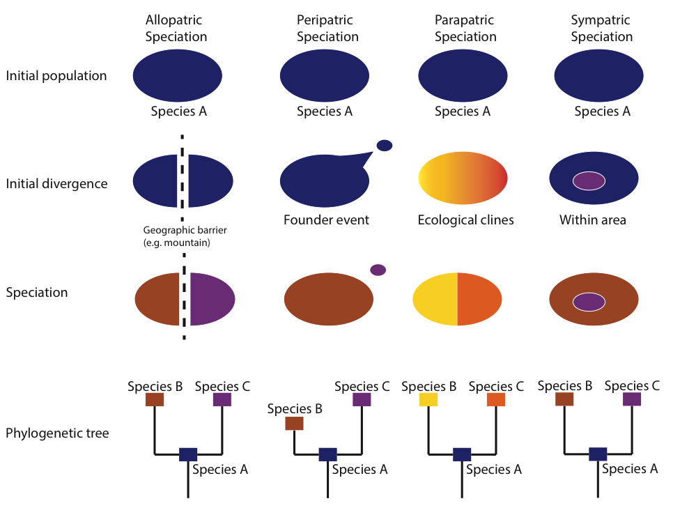
A similar process occurs during founder events, which can be defined as a small subset of individuals in a population colonizing a new location. A good real-world example is the colonization of Madagascar from mainland Africa. Research has shown that the majority of organisms colonized Madagascar by overseas dispersal (versus the continental separation of Africa and Madagascar ~165 Mya). Founder events can lead to what is called founder event speciation, or peripatric speciation. How do these founder events lead to the creation of a new species? Because founder events by definition involve a relative small number of individuals from a parental population, genetic drift will have a pronounced influence on allele trajectories once these individuals colonize a new area (Fig. 6).
")
Similar to population bottlenecks, founder events can lead to the rapid fixation or loss of alleles, in turn increasing the genetic divergence between the parental and founder populations. Other types of speciation include allopatric speciation, which occurs when a geographic barrier (e.g. a mountain range) subdivides an ancestral population, parapatric speciation, which occurs along environmental clines, and sympatric speciation, which occurs without an obvious barrier to gene flow (Fig. 7).
Activity:
1. Simulating the influence of genetic drift
In this lab we will be working with a population genetic simulator called PopG (http://evolution.gs.washington.edu/popgen/). This is a relatively simple, but useful package that can be used to visualize how different microevolutionary processes shape allele frequencies over multiple generations. For simplicity, we will initially examine different processes individually. Go ahead and open the software where you should see a window for specifying certain parameters (see below).
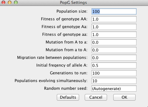
Take a few minutes to familiarize yourself with some of the options. You will notice that there are options to control each of the microevolutionary processes: genetic drift, natural selection, mutation, and gene flow.
Why is genetic drift controlled by the Population Size parameter?
Hit OK to run the default settings. Hopefully you obtain a plot like the one below.
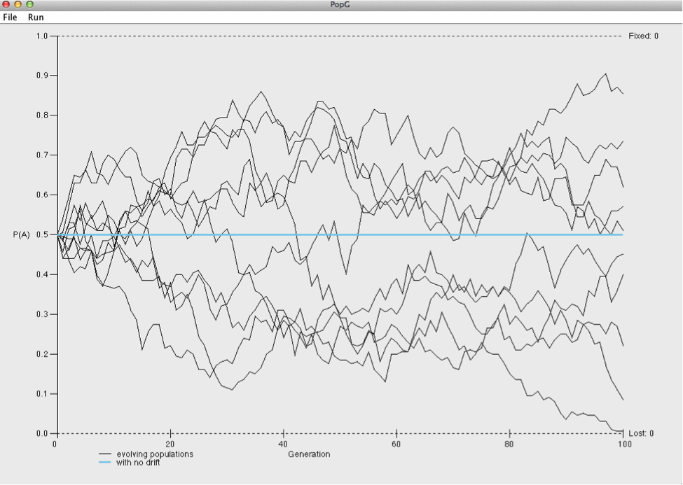
Look at the two axes. The x-axis plots generation number whereas the y-axis shown the frequency of the A allele. Each line is the figure represents a different population (you simulated 10).
How would you explain what is happening in these plots?
Go back to the settings window and change the number of generations from 100 to 1000.
What happened to the A allele in several of the populations?
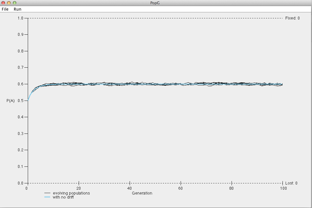
Next, change the population size from 100 to 10000 and run the simulation.
How does the population size parameter influence the frequency of the A allele in each population? Does the A allele become fixed or lost in any population? How does this compare to the simulation using a population size of 100?
2. Simulating the influence of natural selection
Return to the settings window and click the ‘Defaults’ button to restore the default settings. We will now test how natural selection might influence the frequency of the A allele. To minimize the influence of drift in these simulations specify a large population size of 10000. When examining natural selection we usually specify the relative fitness (w) of the different genotypes. By default, a value of 1.0 is assigned to the genotype with the highest fitness, and the remaining genotypes are assigned values relative to the value of 1.0. Let’s start by assigning the following relative fitness values:
wAA = 1.0
wAa = 0.7
waa = 0.3
We can also introduce another parameter called the selection coefficient (s). The selection coefficient is equal to 1 – w. Using the relative fitness values above:
sAA = 1 – 1.0 = 0
sAa = 1 – 0.7 = 0.3
saa = 1 – 0.3 = 0.7
Run the simulation for 10 generations using the relative fitness values above. What happens to the frequency of the A allele?
Next, run the simulation for 100 generations. You should notice that the A allele eventually becomes fixed in each population. At approximately which generation does the A allele become fixed?
In the previous example the homozygous dominant genotype exhibited the highest fitness. What would the simulation look like in a case of overdominance (i.e. heterozygote advantage)? Let’s change the relative fitness values to the following:
wAA = 0.6
wAa = 1.0
waa = 0.4
The selection coefficients in this case would be:
sAA = 1 – 0.6 = 0.4
sAa = 1 – 1.0 = 0
saa = 1 – 0.4 = 0.6
Create a new simulation by first resetting the default parameters. Enter the relative fitness values above to model our example of overdominance. Again, set the population size to 10000 to minimize the influence of drift. Leave all other settings as the defaults.
What do you notice about the frequency of the A allele over the course of 100 generations? What about for 1000 generations? Hopefully your plot looks something like the plot below.
How do your simulations of overdominance compare to your simulations assuming that the homozygous dominant genotype had the highest fitness?
3. Simulating the influence of gene flow
Gene flow is an extremely important microevolutionary process that can introduce new alleles into populations. For example, a beneficial allele lost due to genetic drift may be reintroduced to a population through gene flow. Gene flow can be defined as the successful migration of individuals between populations followed by the transfer of genetic information (i.e. breeding). Studying and quantifying rates and patterns of gene flow has wide-ranging implications for many fields including disease surveillance, human migratory patterns, conservation biology, and systematics. We can use the following equation to determine the change in allele frequency due to migration:
")
where
∆p = the change in allele frequency in the recipient population
m = proportion of migrants within the recipient population
pD = allele frequency of donor population
pR = allele frequency of recipient population
When simulating gene flow it is often interesting to model the interaction between migration and genetic drift. Recall that genetic drift tends to promote the loss or fixation of alleles (leading to reductions in genetic diversity), particularly within small populations. This may lead to large genetic differences between populations, ultimately leading to speciation. Conversely, gene flow can help homogenize populations and maintain a stable number of alleles.
Start a new simulation by restoring the default settings. Click OK to run the simulation for 100 generations. You should see that the frequency of the A allele fluctuates considerably due to genetic drift alone (all other microevolutionary processes were controlled for). What happens if you introduce some migration between each of your 10 populations? Open up the settings window and enter a value of 0.3 for migration rate between populations.
Discuss how the introduction of gene flow influenced allele frequencies of the A allele.
Do you think that gene flow would have a larger or smaller affect on allele frequencies in large populations? Explain your reasoning. It may be useful to perform additional simulations if needed.
4. Simulating the influence of mutation
Mutation is the ultimate source of genetic variation in populations. Mutation can create new alleles in populations, which can then be acted upon by other microevolutionary processes such as drift and selection. It’s important to note that although mutation can create new alleles, it does not substantially alter allele frequencies because mutation is a relatively infrequent event. Mutation rate is commonly represented by the Greek symbol µ and can be expressed in units such as generations or time (e.g. per million years). For example, the typical mutation rate of vertebrate mitochondrial DNA (mtDNA) ranges between about 0.8 – 2.0 substitutions per site per million years. Site refers to a specific base position in an alignment of homologous DNA sequences. Mutation rates of animal nuclear DNA (nDNA) are often an order of magnitude slower. Interestingly, plant mtDNA evolves at a much slower rate than plant nDNA. Thus, different genomes have the ability to provide different amounts of evolutionary information, and target genes can be tailored to one’s specific research objectives. We can use the equation below to calculate the frequency of the A allele after a specific number of generations, assuming we know the starting allele frequency and the mutation rate.
^t = \frac{p_t}{p_0}")
where
µ = mutation rate from the A allele to the a allele
t = time (e.g. number of generations)
pt = frequency of the A allele after t generations
p0 = initial frequency of the A allele
We can rearrange the problem to solve for pt:
^t")
Calculate the frequency of the A allele after 500 generations, assuming a mutation rate of 0.0001 per generation and an initial frequency of 0.5.
Let’s perform some simulations to observe how mutation alters allele frequencies. Setup a new run by first restoring the defaults. To minimize the influence of drift, set the population size to 10000. Enter 0.0001 for the mutation rate from A to a and run the simulation for 500 generations.
What do the results suggest? Would you say that the frequency of the A allele is changing dramatically? Explain your reasoning.
Next, go back to the settings window and enter a rate of 0.001 for the mutation rate from a to A. and rerun the simulation.
How do these results differ from the previous simulation that assumed no mutation from a to A?
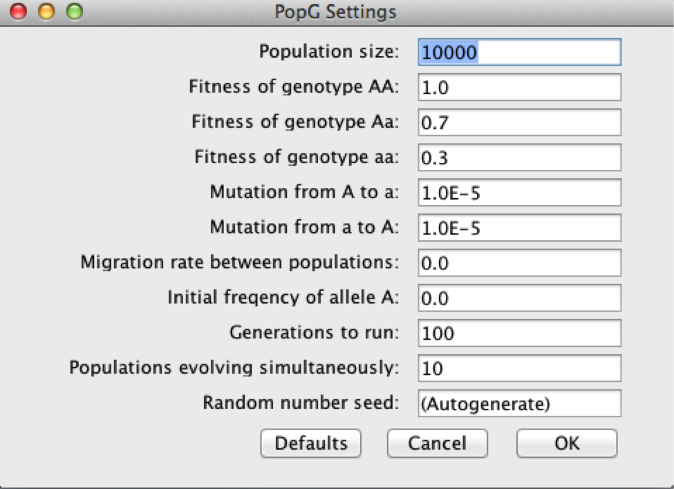
Finally, let’s try to model a situation where mutation creates a new beneficial allele that is acted upon by natural selection. Theory predicts that the beneficial allele should become fixed in a population if the population size is large enough to minimize the affect of drift. In this example, we will assume that the population was originally monomorphic for the a allele, and mutation introduces a beneficial A allele. We will also assume that the mutation rate from A to a is the same as the mutation rate from a to A (0.00001). We will use the following relative fitness values:
wAA = 1.0
wAa = 0.7
waa = 0.3
Your settings should look like the diagram below.
Provide a detailed description of what is happening in your model.
If time permits, perform additional simulations of your choosing, mixing and matching different processes to see how allele frequencies are affected. Upon successful completion of the lab you should be comfortable with how the different microevolutionary processes interact to shape allele frequencies in populations.

