Probability, Statistics, and Measurements

The goal of this laboratory is to provide an introduction to basic concepts and techniques commonly used to study genetics. The first portion of the lab is devoted to the concept of probability and how we can use basic probability theory to understand genetic concepts and crosses. Genetic crosses are commonly used to study patterns of inheritance of traits. A trait, or a character, is generally any observable phenotypic characteristic of an organism such as eye color, skin color, height, etc. Gregor Mendel, often considered the father of genetics, performed many genetic crosses to quantify patterns of inheritance in pea plants. Based on the results of his experiments he came up with three laws:

Law 1: Law of Segregation

Alleles in diploid individuals separate during the process of gamete formation (meiosis).

Remember that a diploid cell contains two sets of chromosomes, one from the father and one from the mother. Thus, each gene will contain two alleles. The alleles can either be the same (homozygous) or different (heterozygous). For example, if we assume that pea pod color (green versus yellow) is controlled by a single gene with two alleles (R and r), RR and rr would represent homozygotes and Rr would indicate a heterozygote. During gamete formation, only one of the two alleles will be passed on to the sperm or egg. In other words, the two alleles segregate from one another (see Fig. 1).

 Law 2: Law of Independent Assortment

Different genes randomly sort their alleles during the process of gamete formation (meiosis).

For example, going back to Mendel’s experiments with pea plants, suppose we are working with two genes we will call Gene 1 and Gene 2. Gene 1 controls pea pod color and consists of two alleles (R = green, r = yellow). We assume that the R allele is dominant, meaning that RR and Rr genotypes produce green pods and rr genotypes produce yellow pods. Now assume that Gene 2 controls seed pod shape and also contains two alleles (Y = constricted, y = round). Assume that Y is dominant over y, such that YY and Yy genotypes produce constricted pods and yy genotypes produce round pods. Mendel’s Law of Independent Assortment states that the alleles at these different genes will sort independently of one another during gamete formation. In other words, the R allele will not always be associated with the Y allele and the r allele will not always be associated with the y allele in each sperm or egg cell. All combinations of alleles are possible (Fig. 1).

 

Law 3: Law of Dominance

A heterozygous individual will express the phenotypic characteristics of the dominant allele.

 For example, in our green versus yellow plant example, we say that the green allele (R) is dominant to the yellow allele (r) because both RR and Rr plants demonstrate the green phenotype.

We will come back to Gregor Mendel and genetic crosses in subsequent labs. First, we will need to understand basic probability theory and how it can be used to predict the likelihood of particular outcomes.

Part 1: Probability and Statistics

Probability can be defined as the chance that any particular outcome will occur. For example, what is the probability of tossing a coin and obtaining heads? The answer would be ½ or 50%. Thus,

 

 

Going back to our coin-flipping example, we asked what the probability would be of flipping a heads on one try. Thus, the numerator (number of times a particular event will occur = 1) and the denominator = 2 (there are only two possible outcomes, heads or tails).

What would be the probability of drawing a black card from a deck of cards on one try? What would be the probability of drawing the King of Hearts from a deck of cards on the first try?

 

 Random sampling error

When calculating probabilities, random sampling error can cause deviations from predicted probabilities. For example, if you tossed a coin six times you would predict that 50% of the tosses would be heads and 50% would be tails. However, it would be possible that you tossed heads twice and tails four times, leading to a high random sampling error and a deviation from the expected value of 50%. Conversely, if you tossed the same coin 1000 times it is highly likely that the number of heads and tails would be closer to 50%. Let’s try this out in a few exercises.

Working in pairs, each group will obtain a deck of cards, a coin, and a dice. For each object, two tests will be conducted, one with a low sample number and one with a high sample number. This will enable us to determine the influence of random sampling error on our outcomes.

Coin test (10 flips)

	Expected	Observed	Difference
Heads
Tails

 

Coin test (100 flips)

	Expected	Observed	Difference
Heads
Tails

 

Cards test (20 cuts)

	Expected	Observed	Difference
Spades
Clubs
Hearts
Diamonds

 

Cards test (100 cuts)

	Expected	Observed	Difference
Spades
Clubs
Hearts
Diamonds

 

Dice test (30 rolls)

	Expected	Observed	Difference
One
Two
Three
Four
Five
Six

 

Dice test (120 rolls)

	Expected	Observed	Difference
One
Two
Three
Four
Five
Six

What can you conclude from these observations? How does sample size influence outcomes with respect to expectations? How do your results compare with other groups?

 

 

 

Although simply visualizing the results in a table can give a sense of how much the observed values deviate from the expected values, statistical tests can provide a more quantitative framework for hypothesis testing. Many statistical analyses require a null hypothesis that assumes no significant difference between treatments, events, or values. For example, in our experiment one null hypothesis would be that there is no significant difference between the expected and observed number of cards in each suit. We can test the null hypothesis using a statistical technique called a chi square (χ²) test. In general, a low χ² is consistent with the null hypothesis, whereas a large χ² might lead us to refute the null hypothesis. How do you know if a value is large enough? First, let’s see how we actually calculate χ². The formula is relatively simple:

where

O = the observed data

E = the expected data based on the null hypothesis

∑ = summation over different categories

 

If we had two categories, the χ² would be calculated as

 

Once we have a χ2 value we need to determine if it is statistically significant. This is accomplished using a χ2 table (see table below). The values inside the table represent calculated χ² values. Before we can either  reject or fail to reject the null hypothesis we need to determine our alpha (P-value) and degrees of freedom (df). P-values can be interpreted in multiple ways. For example, suppose we obtained a χ2 of 0.016 with 1 df. Based on the table, random chance alone would produce a χ2 value greater than 0.016 over 90% of the time (see table below). In most statistical hypothesis testing we adopt an alpha (P-value) of 0.05 or 5%. Examining the table, with 1 df we would need a χ2 > 3.841 (known as the critical value) in order to reject the null hypothesis of no significant difference between observed and expected values. Degrees of freedom is obtained by subtracting 1 from the total number of categories (n – 1). For example, in our cards example df = 3.

Working in groups of two, perform six χ² analyses using the data from the tables above. What can you conclude from your analysis?

 

 

 

 

 

 

 

 

 

The product rule

We can use an approach called the product rule to determine the probability of multiple events occurring. For example, what is the probability of flipping a coin five times and obtaining heads each time? To determine this, we can simply multiply the probability of each independent event occurring:

½ * ½ * ½ * ½ * ½ = 1/32 = 0.03125 = 3.125%

 

What is the probability of drawing a diamond card three times in a row?

 

What is the probability of rolling a six 10 times in a row?

 

What is the probability of flipping heads 20 times in a row?

 

Binomial expansion

Note that the product rule is used to determine the probability of ordered events. It can be used to determine the probability of outcomes in succession. For example, what is the probability of drawing 10 red cards in a row from a standard deck of 52 cards? Conversely, the binomial expansion equation can be used to determine the probability of unordered events. For example, if a couple were to have seven children, what would be the probability that four are boys and three are girls? The binomial expansion equation is as follows:

 

 where P = the probability that the unordered outcome will occur

n = the total number of events.

x = the number of events in one category (e.g. number of males)

p = individual probability of x.

q = individual probability of other category.

 

The symbol ‘!’ represents factorial. For example, 4! = 4 x 3 x 2 x 1 = 24.

 

In this example,

n = 7

x = 4

p = 0.5

q = 0.5

Plugging these numbers into our equation gives us the following:

 

Binomial expansion problem: The disease cystic fibrosis is a recessive disease governed by a single gene. Only individuals homozygous recessive are affected, whereas heterozygous individuals are unaffected carriers. The disease causes difficulty breathing due to the buildup of mucous in the lungs. Suppose two heterozygous parents have five offspring. What is the probability that two of the five offspring will by affected with the disease?

 To solve this problem if will be helpful to first create a Punnett Square depicting the possible genotypes of the offspring. Remember Mendel’s Law of Segregation when constructing the Square and that both parents are heterozygous carriers of the cystic fibrosis allele.

Punnett Square

 

 

 

 

 

What would be the probability that the couple’s first child is affected and the next four children are unaffected? Would you use the product rule or the binomial expansion formula to determine this?

 

 

 

Part 2: Units and dilutions

To adequately work in a genetics or molecular biology lab it is imperative to be comfortable with units of measurement and to be able to convert among units. Most of the time geneticists are working with liquids, so common units of measurement include milliliters (m) and microliters (μ). Below is a table illustrating the different notations.

 

Notation	Factor	Name	Symbol
10-1	0.1	deci	d
10-2	0.01	centi	c
10-3	0.001	milli	m
10-6	0.000001	micro	μ
10-9	0.000000001	nano	n
10-12	0.000000000001	pico	p
101	10	deka	da
102	100	hecto	h
103	1000	kilo	k
106	1000000	mega	M
109	1000000000	giga	G
1012	1000000000000	tera	T

 

Using the table above, make the following unit conversions. Determine this by moving the decimal point the appropriate number of places.

1. 25 μL = __________ mL

 

2. 3 L = ____________ μL

 

3. 150 cL = __________ dL

 

4. 5000 pL = _________ nL

 

5. 75 L = ____________ kL

 

6. 800 nL = __________ cL

 

7. 6 hL = _____________ ML

 

8. 8500 μL = __________ L

 

9. 64 TL = ____________ GL

 

10. 120000 nL = ________ μL

 

In addition to being able to convert among different units of measurement, geneticists also need to make what is called a working stock solution. A working stock solution is a reagent or other solution that is directly used in reactions such as PCR, which we will study later on in the course. Most often, working stock solutions are made by diluting an original stock solution that is at a concentration higher than what is needed for the experiment. By concentration we mean the amount of solutes in a given volume. The concentration of solutes in a solution is usually measured by molarity (M), which is the number of moles per liter of solution (moles/L). For example, 1 M = 1 mole/L. To determine how many grams of a substance is equal to one mole the molecular mass is needed (we will not explore this in this lab). The general formula for making a dilution solution is the following:

 

 

where

C₁ = the original concentration of stock solution

V₁ = the volume of stock solution needed to make working solution

C₂ = the desired concentration of working solution

V₂ = the desired final volume of working solution

 

How would you make a 100 μL working stock at a concentration of 0.5 μM from a stock solution at a concentration of 0.1 mM? Always remember to put everything into the same units first!

 

 

 

 

 

What would be the working stock concentration (in molarity) if you diluted 250 μL of a stock concentration of 10 μM in a total volume of 1 mL?

 

 

Part 3: Biological Controls

In most scientific experiments, a control is needed to make sure that the experiment was successful and to guard against incorrect conclusions. Controls are particularly needed in the field of molecular genetics. As we will learn later in the semester, a technique called polymerase chain reaction (PCR) can be used to amplify (i.e. make many copies of) a particular segment of DNA. The following components are needed to perform PCR:

1. Water
2. PCR buffer
3. dNTP (nucleotides)
4. Primers (oligonucleotides) that flank the region of DNA to be amplified
5. Taq polymerase enzyme
6. DNA

We will discuss how PCR is actually performed later in the semester. For now, let’s think about why controls are needed when we perform these experiments. First, it’s important to understand what we mean by a negative control. In the case of molecular genetics and PCR, a negative control is a sample that we add to our experiment that should not produce a positive reaction. If template DNA is required for successful amplification, we would not expect to see a product from a sample lacking any DNA. Figure 2 below shows a gel image resulting from a PCR with seven real samples (with DNA) and one negative control (water). Note that PCR product (black bands) can be seen for each of the samples, but not the negative control (water). This would be considered a successful run.

 

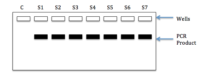
So why is the inclusion of a negative control useful? Suppose that a band was also present in our water sample. This would indicate the presence of DNA contamination of our negative control (water). Since this happened, there might also be contamination of our real samples and therefore the results may be suspect. In general, contamination of the negative control requires that the experiment be conducted again, using a new negative control and possibly new reagents (e.g. water, buffer, primers, dNTPs).

Although not used as frequently as negative controls, some experiments may make use of positive controls. Positive controls are samples that we know should work/amplify using a given set of experimental conditions. If the positive control works, but the samples do not, this would indicate an issue with the samples. If neither the samples nor the positive control amplifies, this may indicate an issue with the conditions and/or reagents used in the experiment. We will make use of both negative and positive controls later on in the semester when we work on the GMO activity.