
As I have been saying over the course of the semester, you should work through the Final Exam Review exercises before the final exam (coming up on Monday Dec 21).
Below is a guide to the exercises/topics on the final exam review sheet, with similar exercises from the quizzes and exams listed. Look at the solutions of the exams and quizzes for further review as you work through the Final Exam Review exercises! (All the solutions have been uploaded here.)
Specifcally, here’s what I recommend you do to prepare for the final:
- Print out the Final Exam Review sheet; you could also print out the quiz and exam solutions
- Go through the outline below and work through each of the Final Exam Review topics (ideally do 2 or 3 topics each day–it’s too much to try do it all in one day!)
- Try to do the Final Review exercise
- If you can’t remember how to do that kind of problem, go through the solutions of the corresponding Quiz and Exam questions
- Then try the Final Exam Review exercise again, using the quiz and/or exam solution as a guide
- To incentivize you to actually do them, I’ve assigned a handful of Final Exam Review exercises for HW#10
#1: Polynomial and rational function inequalities
- Use the graph of the function on the LHS of the inequality to find the interval(s) where the function is greater than or less than 0 (i.e., where the graph above or below the x-axis).
- For inequalities involving a quadratic polynomial, such (a)-(c), solve for the roots of the quadratic by factoring (or by using the quadratic formula). This gives you the x-intercepts of the graph, i.e., it tells you exactly where the graph crosses the x-axis.
- For inequalities involving a rational function, such as (d), solve for the x-intercept (by solving where the numerator equals 0), but you’ll also need to solve for the vertical asymptote (by solving where the denominator equals 0). Then look at the graph of the rational function.
- See Exam 2, #6
#2: Absolute value inequalities
- If the inequality is
, then solve
- If the inequality is
, then solve
and solve
- See Quiz 1, #1 and Exam 1, #1
- See also the video posted here


#3: Rational Functions
- Find the x- and y-intercepts algebraically, the domain, the vertical and horizontal asymptotes (see this post for an outline of how to do all that algebraically!)
- Graph the function using a graphing calculator and the information above
- See Exam 2, #4 & #5
#4: Difference Quotients
- Find
in order to set up and simplify the difference quotient
(in particular for quadratic polynomials, i.e.,
)
- See Quiz 1, #2 and Exam 1, #2
- See also the videos posted here
#5: Polynomials
- Find the roots of a polynomial algebraically (using a combination of techniques: by identifying an integer root at x=c and using long division by (x-c); by factoring; by using the quadratic equation)
- Graph the function using a graphing calculator and the roots
- See Quiz 2, #2 and Exam 2, #3
#6: Vectors
- Find the magnitude and direction angle of a vector
- See Example 22.4 on pp301-302 of the textbook
#7: Skip this since we didn’t have time to cover this topic
#8: Properties of Logarithms
- Simplify logarithmic expressions using the properties of logarithms
- See Quiz 3, #2 and Exam 3, #2
#9: Graphing logarithmic functions
- Finding the domain, asymptote and x-intercept of a logarithmic function, and sketching its graph
- See Quiz 3, #1 and Exam 3, #3
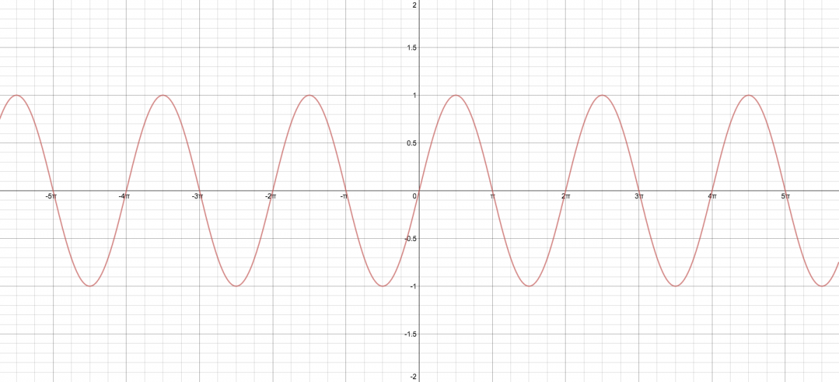
#10: Amplitude, period, phase shift of a trigonometric function
- See Exam 3, #7
#11: Solving trigonmetric equations
- See Exam 3, #6
- Also see this post!
#12 and #13: Exponential population growth
- Write down the function
given the initial population
and the rate r at which the population is growing (or decreasing, as in #12!)
- Solve for the time it takes for the population to grow (or decrease) by a certain multiple (i.e., to double to
)
- See Exam 3, #5
- See also this post
#14: Find the inverse of a given function
- Given y = f(x), switch x and y, and solve for y in terms of x
- See Exam 1, #6 and Quiz #2, #1
#15: Sums of arithmetic sequences
- Given an arithmetic sequence, where each successive term is found by adding a constant “difference” d the previous term (i.e.,
for all i > 1), identify the initial term
and the constant d
- For example: given the sequence
, we see that
and
- For example: given the sequence

- Use the following formulas to calculate the sum of the 1st k terms of the sequence:
- the k-th term of the sequence
is given by the formula
- then use the formula for the sum of the 1st k terms of the sequence:
- the k-th term of the sequence
*d")
")
- For example, to calculate the sum of first 83 terms of the arithmetic sequence
- first we calculate that the 83rd term in the sequence is
and so
- the sum of the first k = 83 terms is
- first we calculate that the 83rd term in the sequence is
 = -11,537")
- See also Example 23.15(c) on pp321-322 of the textbook
- The formulas above are on p318 and p321, respectively
#16: Sums of infinite geometric sequences
- Given a geometric sequence with initial term
for all i > 1), identify the constant r
- Then use the following formula to calculate the sum of an infinite geometric sequence:

- For example, given the sequence
, we see that
, with
- Hence,
, and so
, and thus the sum of this geometric series is
= -6*(3/4) = -18/4 = -9/2.

- See also Example 24.10(c) on pp332-333 of the textbook
#17: Skip this since we didn’t have time to cover this topic
 =7 (1.012)^t")
 = c (1+r)^x") , where c is the initial population.)
, where c is the initial population.) =P_0 (1+r)^t = 2*P_0")
 = \log 2 \Longrightarrow t = \frac{\log 2}{\log (1+r)}")
 (for any integer n). Hence that is the solution set of the equation
 (circled):
 to these two basic solutions.
 and
and
 and
and  (find these points on the unit circle!).
 and
and  (where n = 0, 1, 2, 3, …)
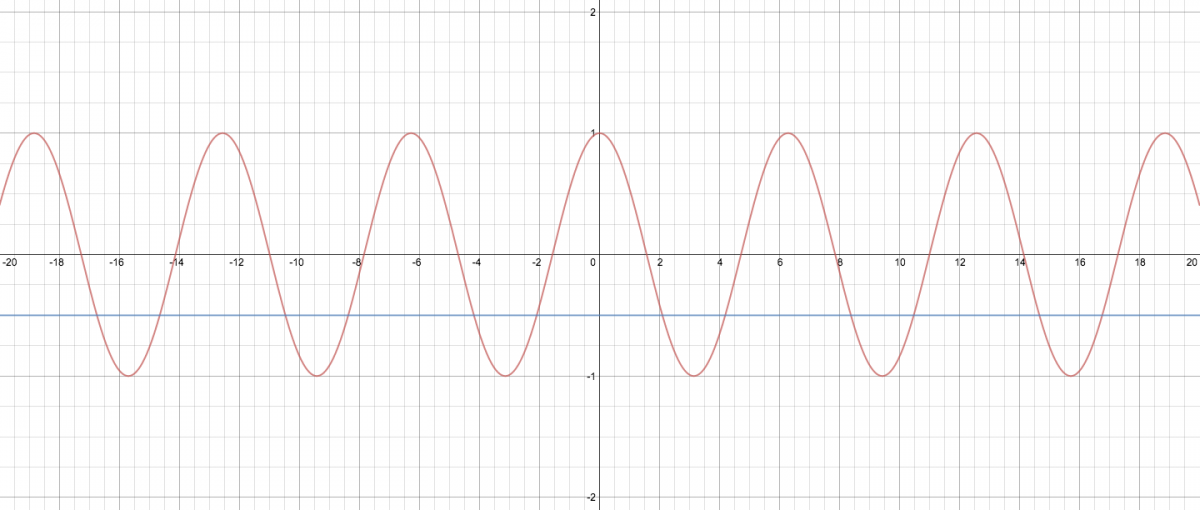

 .
. .
. is at the 0 position until it goes all the way around the circle. You’ll the graphs trace out one full cycle of the sine and cosine waves (i.e., over the interval [ 0, 2 pi].
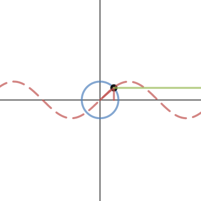

