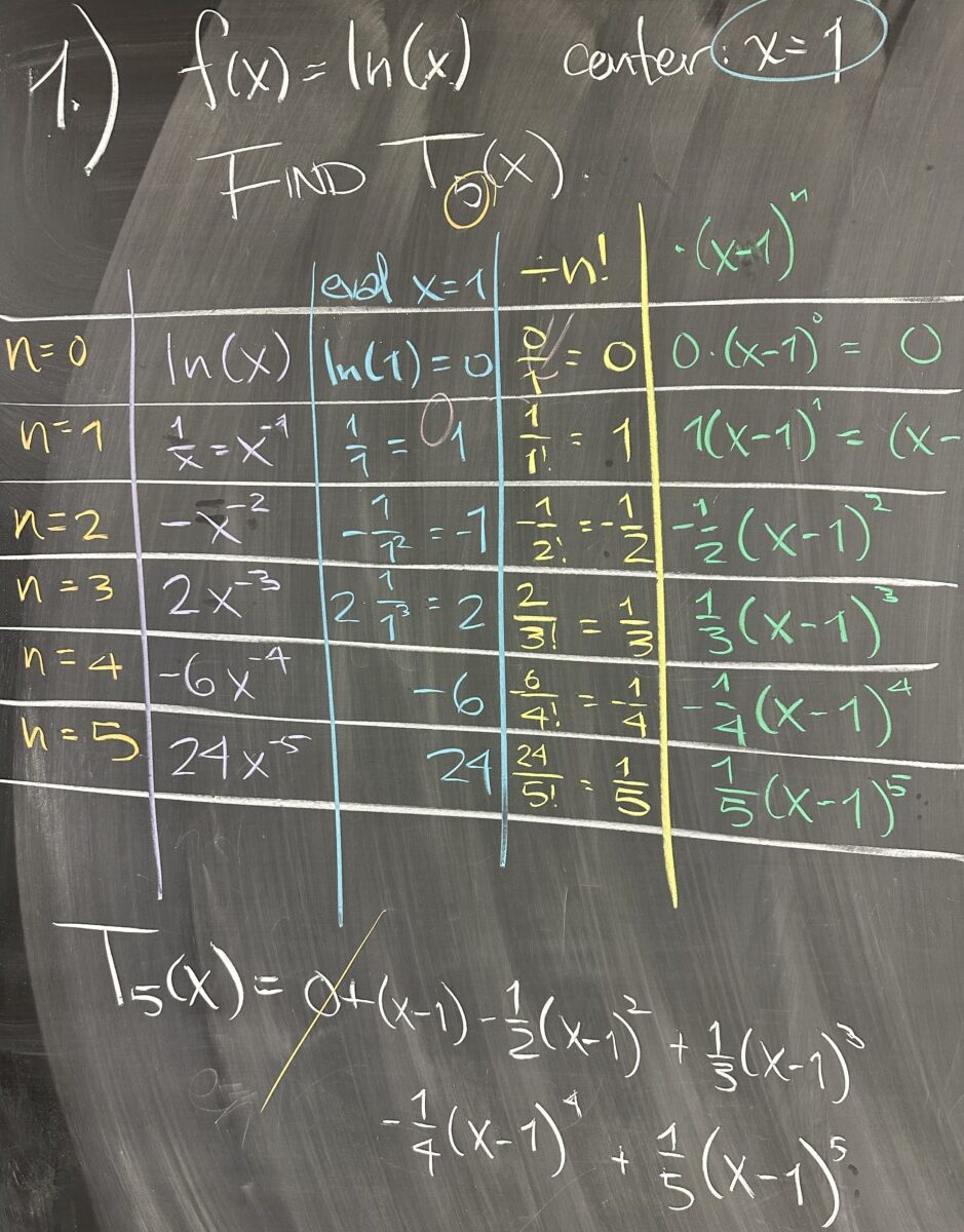
Today’s quiz consisted of a single problem: find the fifth-degree Taylor Polynomial approximation of the function \(f(x)=\ln(x)\) centered at \(x=1\). In setting up for this Taylor Polynomial, we create a table with rows for all values of \(n\) starting at \(n=0\) and ending at the fifth-degree: \(n=5\).
In the first column of the first row we place the function which we are going to approximate: \(f(x)=\ln(x)\). Moving down, row-by-row, we take a derivative and place it in the next row. \[f(x)=\ln(x)\quad f'(x)=\frac{1}{x}=x^{-1}\quad f”(x)=-x^{-2}\quad f^{(3)}(x)=2x^{-3}\quad\ldots\]
In the second column, we take each \(n^{th}\) derivative and evaluate it at \(x=1\). This means the contents of our second column must be numeric (not functions, as in the first column).
Taking the values in each row of the second column, we divide by \(n!\) (where \(n\) is different for each row, of course) and write the result in the third column. Again, this result must be numeric.
In the fourth (and final) column, we use the numeric value from the third column as a coefficient for \((x-1)^n\) (again, \(n\) is different for each row).
Putting it all together, we add the results from the fourth column to create one long polynomial: \[T_5(x)=0+(x-1)-\frac{1}{2}\left(x-1\right)^2+\frac{1}{3}\left(x-1\right)^3-\frac{1}{4}\left(x-1\right)^4+\frac{1}{5}\left(x-1\right)^5\]

The quiz did not go this far, but if we wanted to continue extending this Taylor Polynomial to higher and higher degrees, we would need to know the coefficients for the higher and higher powers of \((x-1)\). In this case (for \(f(x)=\ln(x)\) centered at \(x=1\)), there is a pattern that emerges for these coefficients.
Consider the coefficients as a sequence: \(c_n = \{0,1,\frac{1}{2},-\frac{1}{3},\frac{1}{4},-\frac{1}{5},\frac{1}{6},\ldots\}\). The patterns we see emerging don’t really fit with the \(n=0\) term, \(c_0 = 0\). Since this coefficient ensures that the zero-th term is zero, so we can simply start counting with \(n=1\) and ignore the \(n=0\) term.
Without the first zero term, the patterns we see are the alternation of positive and negative values and each fraction having denominator matching \(n\). Since the alternation is negative for \(n\) even and positive for \(n\) odd, the closed form is \((-1)^{n+1}\). As for the fractions, the closed form is \(\frac{1}{n}\). Together, we see that the coefficients follow the closed form \(c_n = (-1)^{n+1}\frac{1}{n}\).

Since \(c_n\) is the coefficient for \((x-1)^n\) we use summation notation to write the Taylor Series for \(f(x)=\ln(x)\) centered at \(x=1\) as: \[T(x)=\sum_{n=1}^\infty (-1)^{n+1}\frac{1}{n} \left(x-1\right)^n\]
This Taylor Series is a power series, and the usual question for power series is, “what is its interval of convergence?”
Recall from our unit on series that the Ratio Test is the go-to series test for intervals of convergence. Writing out both \(a_n\) and \(a_{n+1}\) we compute \[L = \lim_{n\to\infty} \left|\frac{a_{n+1}}{a_n}\right| = \lim_{n\to\infty} \left|\frac{(-1)^{n+2}}{(-1)^{n+1}}\frac{n}{n+1}\frac{(x-1)^{n+1}}{(x-1)^n}\right| = |x-1|\]

By the ratio test, we know the series will converge if the limit has absolute value less than one. This means \(|x-1| < 1\), which is true whenever \(0<x<2\). Furthermore we know that the ratio test will be inconclusive if the limit has absolute value equal to one. This means \(|x-1| = 1\), which is true if \(x=0\) or \(x=2\) (the “endpoints” of our interval).
Since the Ratio Test is inconclusive for these two \(x\)-values, they must be checked individually using other tests.

When \(x\) is replaced by \(0\), the series reduces to \[T(0)=\sum_{n=1}^\infty (-1)\frac{1}{n} = -1\sum_{n=1}^\infty \frac{1}{n}\]
With the \(-1\) factored out, we see just a p-series with \(p = 1\). By the p-series test, since \(p \leq 1\), we conclude that this series, \(T(0)\), is divergent.

At the other endpoint, replacing \(x\) with \(2\) simplifies to give us an alternating series: \[T(2)=\sum_{n=1}^\infty (-1)^{n+1}\frac{1}{n}\]
The absolute sequence (the non-alternating portion) for \((-1)^{n+1}\frac{1}{n}\) is \(b_n=\frac{1}{n}\). Since we’re applying the Alternating Series Test, we have three conditions to check for \(b_n\): is it positive? is it monotone decreasing? is the limit zero? The answer is “yes” to all three. As such, we can conclude that the series, \(T(2)\) converges.
With \(x=0\) being excluded from the interval of convergence, and \(x=2\) included, the final answer for our interval of convergence is \((0,2]\).

This notion of finding a closed form for the coefficients in a Taylor Series is not always possible. However, we now look at a Taylor Series that has a very straightforward closed form. The Maclauren Series for \(f(x)=e^x\) (remember that “Maclauren” implies centering at \(x=0\)), has coefficients \(c_n=\frac{1}{n!}\) and overall series: \[\sum_{n=0}^\infty \frac{x^n}{n!}\]
Again, considering the interval of convergence for this power series, we turn to the Ratio Test. When we simplify the ratio \(\frac{a_{n+1}}{a_n}\), we get \(\frac{x}{n+1}\) which has limit zero as \(n\) goes to \(\infty\) for any \(x\)-value. As such, the Ratio Test concludes that the series converges for any \(x\)-value. With convergence for all \(x\), the interval of convergence is \((-\infty,\infty)\).

Another function that has a clear pattern in its derivatives is \(f(x)=\sin(x)\). If we consider its Maclauren Series, our pattern of derivatives is a repeating cycle of \(\{0,1,0,-1\}\). Since each of the even terms will have coefficient zero, that leaves a polynomial that consists only of odd-degree terms.
Writing out the first several terms of the Maclauren Series for \(f(x)=\sin(x)\) we get: \[x-\frac{1}{3!}x^3+\frac{1}{5!}x^5-\frac{1}{7!}x^7+\frac{1}{9!}x^9-\ldots\]
There’s an alternation in these coefficients, but under the initial indexing, the alternation occurs in every other even value. (This is unlike the usual alternation that we see between even and odd degrees.) So we re-index the series, starting with \(x\) as the \(n=0\) term, \(\frac{1}{3!}x^3\) as the \(n=1\) term, and so on.
Under the new index, we see that the degree (as well as the factorial) is \(2n+1\). Also notice that the alternation is back to even vs. odd degrees with the even terms being positive and the odd terms being negative. Putting both of these patterns in combination with the new index, we write the Maclauren Series as \[T(x) = \sum_{n=0}^\infty (-1)^n\frac{x^{2n+1}}{(2n+1)!}\]

If we follow the same strategy for the Maclauren Series of \(f(x)=\cos(x)\), we note that the derivatives follow the cycle \(\{1,0,-1,0\}\). This cycle causes the odd-degree terms to have coefficient zero, leaving only the even-degree terms.
Again, we write out the first several terms in order to attempt a re-indexing: \[1-\frac{1}{2!}x^2+\frac{1}{4!}x^4-\frac{1}{6!}x^3+\frac{1}{6!}x^3-\ldots\]
Re-indexing, starting with \(1\) as the \(n=0\) term, we see the power and factorial both following the pattern \(2n\), and the alternation starting with positive when \(n=0\). This allows us to write the series as: \[T(x)=\sum_{n=0}^\infty (-1)^n\frac{x^{2n}}{(2n)!}\]


Recent Comments