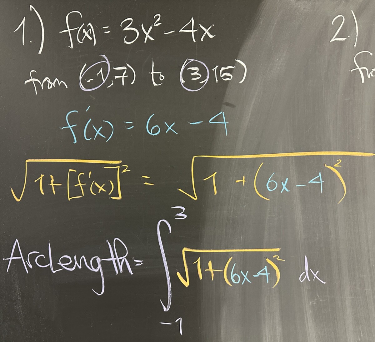
Today’s quiz contained three questions about arc length. The entire problem consisted of setting up (but not evaluating) the integral for arc length of the given functions. Recall that the arc length of \(f(x)\) from \(x=a\) to \(x=b\) is calculated using the integral: \[L = \int_a^b \sqrt{1+\left[f'(x)\right]^2}\,dx\]
In the first problem, we are given \(f(x)=3x^2-4x\) and the points \((-1,7)\) and \((3,15)\). Right away it should be clear that our bounds for \(x\) are \(-1\leq x\leq 3\). Then we must construct the integrand: \(\sqrt{1+\left[f'(x)\right]^2}\).
Once we determine \(f'(x)\), the rest is pretty straightforward. So \(f'(x)=6x-4\) and as a result: \[L = \int_{-1}^3 \sqrt{1+\left(6x-4\right)^2}\,dx\]

The second problem follows the same structure using \(g(x)=7\sqrt{x^3}\). From the given points, we determine that \(0\leq x\leq 4\) and then we find \(g'(x)=\frac{21}{2}\sqrt{x}\).
Putting it all together: \[L = \int_0^4 \sqrt{1+\left[\frac{21}{2}\sqrt{x}\right]^2}\,dx\]

Finally, the third problem is again the same structure with \(h(x)=5\cos(2x)\). From the given points, we determine that \(0\leq x\leq\pi\) and then we find \(h'(x)=-10\sin(2x)\).
Putting it all together: \[L = \int_0^\pi \sqrt{1+\left[-10\sin(2x)\right]^2}\,dx\]

Today’s topic deals with extending the idea of linear approximation from Calculus I. In Calc I, a common question is finding an equation for the line tangent to a given function at a given point. We also learn that tangent lines are “very close” approximations of the given function whenever \(x\) is also “very close” to the point of tangency.
Recall that the formula for the linear approximation of \(f(x)\) at \(x=a\) is given by: \[L(x) = f'(a)\left(x-a\right)+f(a)\]

In this lesson, we begin to extend this idea of linear approximation to use higher degree terms (in order to hopefully get a “better” approximation). Naïvely, we might look at the pattern of coefficients and deduce that each comes from higher derivatives of our original function — and in each degree, simply increase the power on \((x-a)\) by one.
We followed this naïve approach for the function \(f(x)=x^2-5x+6\), and ended up with \(2x^2-5x+6\) as our approximation. This approximation looks close to the original \(f(x)\) on paper, but is actually a poor approximation because the coefficient of the \(x^2\) term is not good.
The problem here is that we are attempting to infer a pattern from only two initial terms. With linear approximation, there is only the degree zero term: \(f(a)\), and the degree one term: \(f'(a)\left(x-a\right)\). Using notation from sequences and series, we will use \(n\) to represent the degree for each term. It seems like we want the \(n\)-th derivative evaluated at \(a\) as our coefficient, but in actuality, we need to tweak this value by dividing by the factorial of the degree: \(\div n!\).
This extra step to the pattern is not evident in the first two terms because in degree zero, \(n=0\), which has factorial \(0!=1\), and in degree one, \(n=1\), which also has factorial \(1!=1\). In both cases, division by the factorial of the degree results in no change to the coefficient. However, in the degree two term \(n=2\), division by \(2!=2\) would have caused our original (naïve) approximation to end up being \(x^2-5x+6\).
Note that our second-degree approximation of the original \(f(x)\) (which was itself a second-degree polynomial) is actually now identical to the original \(f(x)\) with this change in coefficient pattern.

This polynomial approximation using derivatives is called the “Taylor Series” for \(f(x)\), “centered” at \(x=a\). As we have already seen, this process builds up a polynomial approximation — one degree at a time.
Formalizing the pattern requires some recollection of notation from Calculus I. Since we will be taking higher derivatives of our original function, we’ll need to remember that the \(n\)-th derivative of \(f(x)\) is denoted \(f^{(n)}(x)\), and when evaluated at \(x=a\), is denoted \(f^{(n)}(a)\).
Division by \(n!\) (where \(n\) is the degree) gives us \(\frac{f^{(n)}(a)}{n!}\), and finally multiplying by \(\left(x-a\right)^n\) gives us the following expression for our “degree \(n\) term” for the Taylor Series approximation of \(f(x)\) centered at \(x=a\): \[\frac{f^{(n)}(a)}{n!}\left(x-a\right)^n\]
To construct the entire Taylor Series (all degrees!), then, we must simply add together the terms from each degree. Notationally, we will use what we learned from series to represent this sum over \(n\), the degree, starting from \(n=0\): \[T(x) = \sum_{n=0}^\infty \frac{f^{(n)}(a)}{n!}\left(x-a\right)^n\]
If we do not (or cannot) compute all degrees for the Taylor Series, we must have stopped at some “highest” degree. In such cases, we use the terminology “Taylor Polynomial”. Note here that the word “series” refers to infinite sums (no “highest” degree, \(n\) increases forever), while the word “polynomial” refers to a finite sum (with some “highest” degree).
Taylor Series are often labeled as \(T(x)\), while Taylor Polynomials are labeled with their degree — for example, a fifth-degree Taylor Polynomial would be labeled as \(T_5(x)\).
Computation for a Taylor Polynomial (or Series) is an involved process. We must perform the same calculations for each degree. For each value of \(n\), we need the \(n\)-th derivative as a function, then we need to evaluate that derivative at \(x=a\). Then we must divide by the factorial of the degree, \(n!\), and finally multiply by \((x-a)^n\).
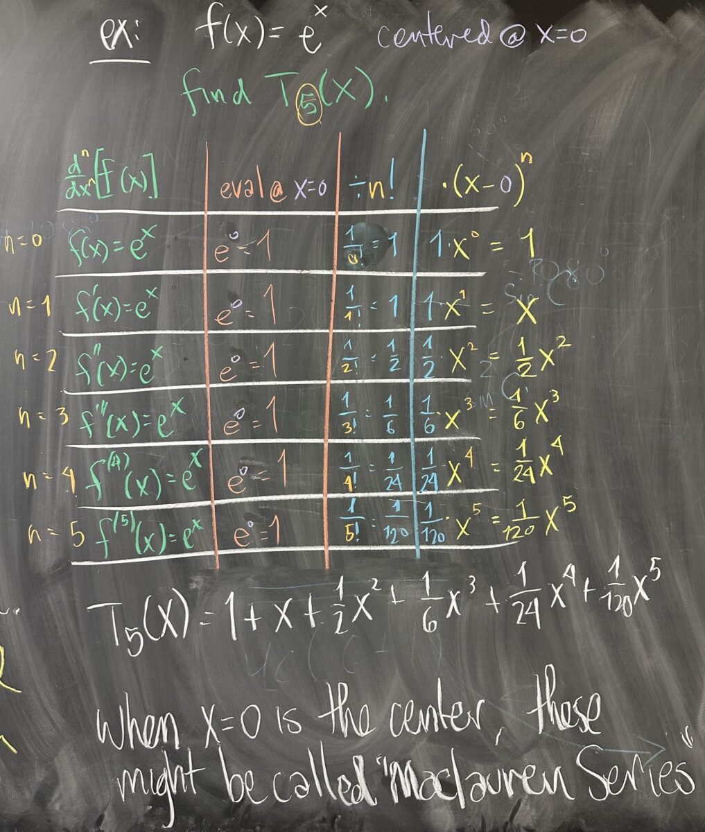
It is recommended that you create a table for your calculations. In this table, you will have one row for each degree, starting at \(n=0\), then \(n=1\) and so on, with a final row for your “highest” degree. In this example, we compute \(T_5(x)\), the \(5^{th}\) degree Taylor Polynomial for \(f(x)=e^x\), centered at \(x=0\).
Since we want the \(5^{th}\) degree polynomial, that means 6 rows in our table starting at \(n=0\) and ending at \(n=5\). In each row, our first column is the \(n\)-th derivative of \(f(x)\). The first row is the \(0^{th}\) derivative, which is just the original function. Proceed down the rows along the first column, each time taking another derivative of the function in the preceding row. This is straightforward for \(f(x)=e^x\) since \(\frac{d}{dx}\left[e^x\right] = e^x\).
Then begin a new column where we will take each derivative from the first column and evaluate it at \(x=0\), (our “center”). Do this for each row, resulting in a single numerical value for each row in the second column.
For the third column, we take the result from the second column and divide by \(n!\). Note that \(n\) has a different value in each row, so pay close attention! Since we’re dividing a numerical value by another numerical value, our third column should again result in a numerical value for each row in the third column.
In the fourth (and final) column, multiply the value from the third column by \((x-a)^n\). Again, take note that \(n\) has a different value in each row, so you should be seeing higher powers of \((x-a)\) as you go down each row in the table. Also note that in our example, the center is \(x=0\), which means that we can simplify \((x-0)^n = x^n\).
This is the last step in the algorithm to construct the Taylor Polynomial: add up the results from our final column: \[T_5(x) = 1+x+\frac{1}{2}x^2+\frac{1}{6}x^3+\frac{1}{24}x^4+\frac{1}{120}x^5\]
In conclusion, it is important to note that Taylor Series and Polynomials centered at \(x=0\) are sometimes referred to as “Maclauren Series” or “Maclauren Polynomials”. Whenever you encounter “Maclauren” Series or Polynomials, the center will not be stated explicitly, but it is understood that \(x=0\) is implied to be the center.


Recent Comments