Category: Examples & Explanations (Page 1 of 3)

The application of exponential functions to compound interest is discussed in Sec 17.2 of the textbook, and we discussed in class how compound interest and population growth can in some cases be modeled with exponential functions of the form:

A(t) = P*(1+r)^t

where

Note that in cases like this, we have an exponential function with base b = 1 + r.

For example, we went through this example from the WebWork (Exponential Growth and Decay – Problem 3):

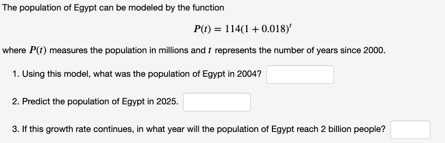
In this case, the initial population (i.e., in the year 2000) is 114 (million), and the growth rate r = 0.018 (i.e., the population grows by 1.8% each year).

We solve (1) by evaluating P(4) (since “P(t) represents the number of years since 2000″):

P(4) = 114*(1.018)^4 = 114*(1.0739674398) = 122.432287359

But note that “P(t) measures the population in millions” so the population is 122.432287 million, and to find the actual population in 2004 we need to multiply this result by 1,000,000 (and round down), so we get 122, 432, 287.

For (2), we similarly evaluate P(25).

For (3), we need to find the value of t such that P(t) = 2000 (since 2 billion is equal to 2000 million). That means we need to solve the following exponential equation:

P(t) = 114*(1.018)^t = 2000

We previously discussed how to solve such an exponential equation by using logarithms and the logarithmic properties. First we divide both sides by the leading coefficient 114:

(1.018)^t = 2000/114

Then we take the logarithm of both sides (we can use any log function; here let’s use “log” i.e., the logarithmic function with base 10):

log [(1.018)^t] = log [2000/114]

Now we apply the log property to bring the variable t down in front–this is what allows us to solve for t!

t*log [1.018] = log [2000/114]

and so

t = log [2000/114]/log [1.018] = 160.57

where we use a scientific calculator with the “log” function to calculate to a decimal approximation.

So it takes approximately 160.57 years for the population to 2 billion. To answer the question of in what year will the population reach 2 billion, we add this number to 2000, to get 2160.57, meaning the answer is the year 2160.

---

Now let’s consider a slightly different form of exponential growth or decay, as described in Exponential Growth and Decay – Problem 1:

So in certain applications, including “interest compounded continuously”, we use an exponential function of the form

A(t) = Pe^rt

In these exponential functions, we use the number e as the base, and the the growth (or decay) rate goes in the exponent (but we still have the initial amount P = A(0) as the leading coefficient of the function.)

Let’s do an example with continuously compounded interest. Here is a version of Problem 2 from the WebWork:

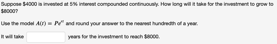
The first step is to put the given values of the parameters into the function:

The value of the coefficient P is the initial amount invested:

P = 4000

and the interest rate of 5% tells us that r = 0.05.

Thus, the function we use here is

A(t) = 4000e^0.05t

Now we can solve for how many years it takes for the investment to grow to $8000, by solving the exponential equation:

A(t) = 4000e^0.05t = 8000

(Note that we are solving for how long it takes for the initial amount to double; this is often called “the doubling time.”

The technique for solving this is similar to what we did in the last part of the population growth example. First divide by 4000 to get:

e^0.05t = 8000/4000

e^0.05t = 2

Now again we take the logarithm of both sides–since we have an exponential function with base “e” here, it makes sense to use the natural logarithm “ln” (i.e., the logarithm with base e!):

ln (e^0.05t) = ln 2

0.05t * ln (e) = ln 2

Now we can see why it’s most convenient to use the natural log; because ln (e) = 1.

So the equation above simplifies to

0.05t = ln 2

and

t = (ln 2)/0.05

We can use a scientific calculator to get a decimal approximation for this value of t.

Here is a useful image of the unit circle labeled with the “special angles” and the coordinates of the corresponding points on the unit circle:

(via http://etc.usf.edu/clipart/43200/43215/unit-circle7_43215.htm)

This image of the unit circle is useful since you can use it to find the sine and cosine of any of the given angles, using the definitions of sin t and cos t as the y- and x-coordinates, respectively, of the point on the unit circle corresponding to the angle t:

See below for a guide to the various WebWork sets on exponential and logarithmic functions. We spent most of class on Mon Nov 30 doing examples from these WebWork sets, so you can also see the recording of that class session on Blackboard, and/or the whiteboard for that class.

“Exponential Functions – Graphs”:

This is an introduction to exponential functions, i.e., functions of the form
f(x) = A*B^x
and their graphs. We discussed the basic shapes of these graphs for various values of the “base” B in class. You should be able to do these exercises with the help of Desmos. One important feature of exponential functions to remember is:
f(0) = A*B⁰ = A
so the y-intercept of any exponential function is at (0, A).

Example: Exponential Functions – Graphs: Problem 6

Note that since the graph slopes down from left to right, we know that the base B has a value between 0 and 1, i.e., 0 < B < 1.

Here the given y-intercept (0,4) gives us the value of the coefficient A:

f(0) = A*B⁰ = A = 4

and then we can use the fact that (1,3) is on the graph to solve for the base B. Since (1,3) is on the graph, f(1) = 3, giving us the equation:

f(1) = A*B¹ = 4*B = 3

and therefore B = 3/4. Thus:

f(x) = 4*(3/4)^x

Extra credit: Problems 8 & 9

“Logarithmic Functions – Graphs”

This introduces logarithmic functions and their graphs as the inverses of the exponential functions. In particular, many of these exercises discuss the domain, the vertical asymptote, and the x-intercept of various log functions. Read the text of Problems 1 & 3 carefully (which we discussed in class), and then use those ideas together with Desmos to work through the other exercises.

Example: Consider the function f(x) = log₃ (-3x – 4).

Domain: Any log function can only take positive values as inputs (see the text of Problem 1!), and so the domain of this function is -3x – 4 > 0, i.e., x < -4/3.

x-intercept: To find the x-intercept, we need to solve f(x) = log₃ (-3x – 4) = 0.
This occurs when -3x – 4 = 1, i.e., at x = -5/3. So the x-intercept is at (-5/3, 0).

Asymptote: Any log function has a vertical asymptote where the input value is 0, so in this case where -3x – 4 = 0, i.e., x = -4/3.

Extra credit: Problems 6 & 7

“Logarithmic Functions – Equations”

This set uses the fact that the definition of the log function y = log_b(x) as the inverse of the exponential function with base b means

y = log_b(x) is equivalent to b^y = x

Use this to rewrite the various logarithmic equations in the exercises as exponential equations!

Extra credit: Problems 5 & 6 (these exercises use the logarithmic properties, which are covered in the “Logarithmic Functions – Properties” set; so you may want to do that set first!)

“Logarithmic Functions – Properties”

This set introduces and applies the basic logarithmic properties. Refer to the textbook (Ch 14, specifically pp199-201) or the first part of Lesson 14 for a list of the basic log properties (which you have to give in Problem 1), and a lot of similar examples. See also the whiteboard for some examples we did in class.

“Exponential Functions – Equations”

This set involves using logarithms to solve exponential equations (i..e, equations in which the variable in the exponent). The key idea is to take the logarithm of both sides of a given equation, and to use the log properties “to bring the exponent down in front”. Refer to the textbook (Sec 14.2) and the latter part of Lesson 14 for examples. See also the whiteboard for some examples we did in class.